Basic Economic Concepts
Contents: 9 sections
Scarcity and opportunity cost
Resources are scarce while wants are unlimited, so every choice involves a trade-off. The opportunity cost of a decision is the value of the next best alternative given up.
Scarcity is what forces every society to answer three questions, what to produce, how to produce it, and for whom, and the scarce resources themselves are the factors of production:
| Factor | What it is | Its payment |
|---|---|---|
| Land | Natural resources | Rent |
| Labour | Human effort | Wages |
| Capital | Tools, machinery, buildings used to produce other goods | Interest |
| Entrepreneurship | Organising the others and bearing risk | Profit |
The payments column matters in Unit 5, where each of these becomes a factor market with its own price.
AP readers expect opportunity cost expressed as a specific forgone alternative, not as "money spent". "The opportunity cost is 2 tractors" earns the point; "the opportunity cost is $400" usually does not.
Two refinements that show up in free-response questions:
- Explicit costs are out-of-pocket payments; implicit costs are the value of resources you already own and give up by using them here. Economic cost = explicit + implicit.
- Economic profit = total revenue − economic cost, so it is always less than accounting profit. Zero economic profit means the firm is earning exactly what its resources could earn elsewhere, a normal return, not "no profit". This distinction returns in Unit 3 and is worth fixing now.
Sunk costs are irrelevant to a rational decision. Money already spent cannot be recovered, so it should not affect the choice about the next unit.
The production possibilities curve
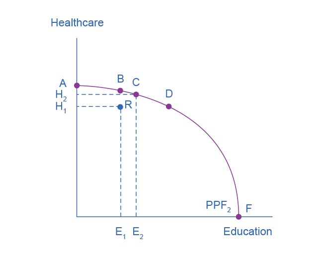
The PPC shows the maximum combinations of two goods an economy can produce with its current resources and technology.
| Position | Meaning |
|---|---|
| On the curve | Efficient: all resources fully and productively employed |
| Inside the curve | Inefficient: unemployment or idle capacity |
| Outside the curve | Unattainable with current resources and technology |
The shape carries information, and AP tests it directly:
- A bowed-out (concave) PPC shows increasing opportunity cost. As you produce more of one good; you must draw in resources progressively less suited to it, so each extra unit costs more of the other good.
- A straight-line PPC shows constant opportunity cost, which implies resources are equally suited to both goods.
Efficiency has two senses worth separating now, because both return in Unit 3. Productive efficiency means being on the curve, nothing is wasted. Allocative efficiency means being at the particular point on the curve that society most values. Every point on the frontier is productively efficient; only one is allocatively efficient.
Shifts versus movements:
- Movement along the curve = reallocating between the two goods; opportunity cost is being paid.
- Outward shift = economic growth from more or better resources, improved technology, or a larger labour force.
- Shift on one axis only = an improvement affecting just one good. This is a frequent FRQ instruction and a frequent lost point: if technology improves in wheat only, the wheat intercept moves and the tractor intercept does not.
Note that a movement from inside the curve to a point on it is not growth in capacity; it is recovering from inefficiency. AP distinguishes these carefully.
Comparative advantage and gains from trade
- Absolute advantage: producing more of a good with the same resources.
- Comparative advantage: producing a good at a lower opportunity cost.
Comparative advantage, not absolute advantage, determines the pattern of trade. A country can hold an absolute advantage in both goods and still gain by specialising, because it cannot hold a comparative advantage in both: the two opportunity costs are reciprocals, so whichever good one party is relatively better at, the other is relatively better at the remaining one.
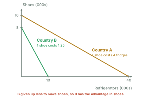
The figure is the argument in one picture. The US can produce more of both goods, so it holds an absolute advantage in both. But its frontier is much flatter: one shoe costs it 4 refrigerators, while in Mexico one shoe costs only 1.25 refrigerators. Mexico is therefore the lower-opportunity-cost producer of shoes, and the US of refrigerators. The point drawn just beyond each frontier is what each country consumes after specialising and trading, a combination neither could reach alone.
Calculating it
Always compute opportunity cost per unit for both parties before concluding. The reliable method: put the good you want the cost of on the bottom of the fraction.
Opportunity cost of 1 wheat = (units of cloth given up) ÷ (units of wheat gained)
Check which kind of problem you have. AP sets two, and they invert the arithmetic:
- Output problems give what each party can produce with fixed resources. Divide the other good by your good.
- Input problems give the resources needed per unit of output. Here the party needing fewer inputs has the absolute advantage, and the cost ratio flips relative to the output case.
A check that catches most errors: the party with the comparative advantage must be the one that gives up less of the other good.
Worked example
Country A can produce 20 cloth or 10 wheat. Country B can produce 40 cloth or 10 wheat.
A: 20 cloth ÷ 10 wheat = 2 cloth per wheat
B: 40 cloth ÷ 10 wheat = 4 cloth per wheat
B has an absolute advantage in cloth and ties in wheat. But A gives up only 2 cloth per wheat while B gives up 4, so A has the comparative advantage in wheat and should specialise in it; B specialises in cloth.
Terms of trade must lie between the two opportunity costs, here, between 2 and 4 cloth per wheat. At 3 cloth per wheat, A receives more than its own cost of 2 and B pays less than its own cost of 4, so both gain.
Confirm from the other side, since the exam may ask for either good:
A: 10 wheat ÷ 20 cloth = 0.5 wheat per cloth
B: 10 wheat ÷ 40 cloth = 0.25 wheat per cloth
B gives up less wheat per cloth, confirming B's comparative advantage in cloth. The two calculations must agree; if they do not, one fraction is upside down.
Marginal analysis
Rational decision-makers act while marginal benefit ≥ marginal cost, and stop where MB = MC.
This single rule underpins nearly every model in the course: the firm produces where MR = MC (Unit 3), hires where MRP = MRC (Unit 5), and society's optimum is where MSB = MSC (Unit 6). Recognising them as one idea makes the rest of the course substantially easier.
Diminishing marginal utility
Utility is satisfaction. Marginal utility (MU) is the extra satisfaction from one more unit.
The law of diminishing marginal utility: as more of a good is consumed, the extra satisfaction from each additional unit falls. The second slice of pizza is worth less than the first.
Two consequences worth holding on to:
- Total utility still rises while MU is positive, it rises more slowly. Total utility falls only once MU turns negative.
- This law is why the demand curve slopes downward. If each extra unit is worth less, a buyer will only take more at a lower price. Unit 2's demand curve is this law drawn sideways.
Utility maximisation
A consumer maximises utility when the marginal utility per dollar is equal across all goods, with the whole budget spent:
MU₍x₎ ÷ P₍x₎ = MU₍y₎ ÷ P₍y₎
If one ratio is higher, shifting spending towards that good raises total utility, so the consumer is not yet optimising.
Second worked example: spending a budget
A consumer has \$24. Good X costs \$2; good Y costs \$4.
| Unit | MU of X | MU₍x₎/P₍x₎ | MU of Y | MU₍y₎/P₍y₎ |
|---|---|---|---|---|
| 1 | 20 | 10 | 40 | 10 |
| 2 | 16 | 8 | 32 | 8 |
| 3 | 12 | 6 | 24 | 6 |
| 4 | 8 | 4 | 16 | 4 |
| 5 | 4 | 2 | 8 | 2 |
Buy in descending order of utility per dollar, not of utility. Working down the ratios, 10, then 8, then 6, then 4, the consumer takes the first four units of each good:
Spending = (4 × \$2) + (4 × \$4) = \$8 + \$16 = \$24, exactly the budget.
Check the condition holds: at 4 units of each, MU₍x₎/P₍x₎ = 8 ÷ 2 = 4 and MU₍y₎/P₍y₎ = 16 ÷ 4 = 4. Equal, with the budget exhausted; this is the optimum.
Total utility = (20 + 16 + 12 + 8) + (40 + 32 + 24 + 16) = 56 + 112 = 168
Why no other bundle beats it. The only other combination that spends exactly \$24 is 2 units of X and 5 of Y:
Total utility = (20 + 16) + (40 + 32 + 24 + 16 + 8) = 36 + 120 = 156
That is 12 utility worse, and it fails the condition: the fifth Y returns 8 ÷ 4 = 2 per dollar while a third X would have returned 12 ÷ 2 = 6. The consumer over-bought Y precisely because Y has the higher marginal utility at every unit, which is the trap. The rule is not "buy the good with the higher marginal utility" but "buy the good with the higher marginal utility per dollar", because Y also costs twice as much.
Economic systems and property rights
Market, command and mixed systems answer what, how and for whom to produce. Markets answer through prices and profit signals; command economies through central planning; mixed economies through both.
Well-defined property rights give owners the incentive to maintain and use resources efficiently, and to trade them to whoever values them most. Where property rights are absent or unenforceable, resources tend to be over-used and under-maintained, the basis of the common-resource problem in Unit 6. This is an AP-specific emphasis with no close counterpart in most other syllabuses.
Common exam mistakes
- Calling a point outside the PPC "inefficient"; it is unattainable.
- Confusing absolute with comparative advantage when assigning specialisation.
- Inverting the opportunity-cost fraction, or treating an input problem as an output problem.
- Stating opportunity cost in dollars rather than as the forgone good.
- Forgetting that a bowed-out PPC implies increasing opportunity cost.
- Shifting the whole PPC when technology improves in only one good.
- Treating zero economic profit as "making nothing"; it is a normal return.
- Including sunk costs in a marginal decision.
- Maximising utility by comparing MU instead of MU per dollar.
- Saying total utility falls whenever marginal utility falls. It falls only when MU is negative.
- Giving terms of trade outside the range between the two opportunity costs.
Exam technique
Label PPC axes with the two goods by name, not X and Y, and mark specific points before explaining anything. An unlabelled axis loses the point even when the shape is right.
In comparative-advantage questions, show the division. Writing "20 ÷ 10 = 2 cloth per wheat" earns credit for method even if the conclusion slips; asserting the answer earns nothing if it is wrong. Build the four-number table first, then compare.
For utility questions, add a MU per dollar column to whatever table you are given before deciding anything. Almost every error in these questions comes from comparing raw marginal utilities across goods with different prices.
When asked to show growth, decide first whether the question describes more resources (whole curve shifts) or an improvement in one good (one intercept moves).
Quick revision
- Scarcity → choice → opportunity cost, stated as a forgone alternative.
- Factors: land, labour, capital, entrepreneurship, earning rent, wages, interest, profit.
- Economic cost = explicit + implicit; zero economic profit = a normal return.
- Sunk costs are irrelevant to marginal decisions.
- On the PPC = efficient; inside = inefficient; outside = unattainable.
- Bowed-out PPC = increasing opportunity cost; straight-line = constant.
- Productive efficiency = on the curve; allocative efficiency = the best point on it.
- Comparative advantage = lower opportunity cost, and it drives trade.
- Terms of trade lie between the two parties' opportunity costs.
- Diminishing marginal utility is why demand slopes down.
- Optimise where MB = MC; consumers where MU/P is equal across goods, budget spent.
What the syllabus asks for on this topicWhat this unit covers
What this unit covers
- Scarcity, choice and opportunity cost.
- The production possibilities curve (PPC).
- Comparative advantage, absolute advantage and gains from trade.
- Economic systems and the role of property rights.
- Marginal analysis, diminishing marginal utility and the cost–benefit principle.
Related AP Economics topics
Not the topic you were looking for? Describe what you are stuck on in your own words and we will take you to the notes that answer it.