National Income and Price Determination
Contents: 8 sections
Aggregate demand
AD shows total planned spending on domestic output at each price level:
AD = C + I + G + (X − M)
- C, consumption. Much the largest component. Driven by disposable income, wealth, consumer confidence and interest rates.
- I, investment. Spending by firms on capital, plus changes in inventories. Note the economist's meaning: buying shares is not investment in this sense. Driven by the real interest rate, expected profitability and business confidence.
- G, government spending. On goods and services. Transfer payments are excluded, because they are not payment for output, they affect AD only once the recipient spends them, which shows up in C.
- X − M, net exports. Driven by foreign income, relative price levels and the exchange rate.
Why AD slopes downward, three effects, and none of them is substitution between goods. That reason works for a single market but not when all prices change together:
- Wealth effect: a lower price level raises the real value of money holdings, so spending rises.
- Interest-rate effect: a lower price level reduces money demand, lowering interest rates and raising investment.
- Exchange-rate (net exports) effect: a lower domestic price level makes exports cheaper and imports dearer, raising net exports.
A change in the price level causes a movement along AD. Anything else shifts it: consumer or business confidence, taxes, government spending, foreign income, exchange rates, wealth, and the real interest rate.
Aggregate supply
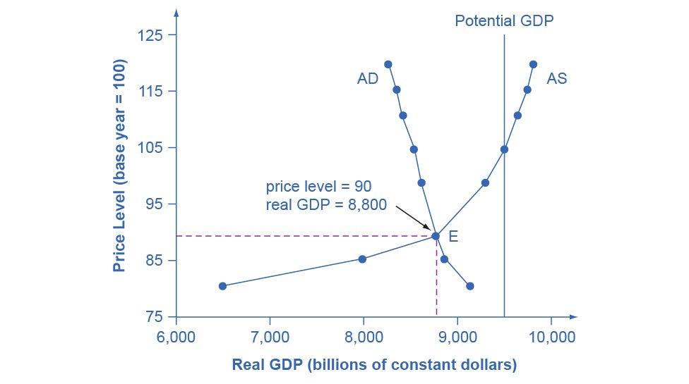
SRAS slopes upward because input prices, especially wages, are sticky in the short run. Wages are fixed by contracts and by expectations formed before the price level changed. So when the price level rises while wages stay put, the real wage falls, margins widen, and firms find it profitable to produce more.
That single assumption, sticky nominal wages, is what creates the entire short run in this course. It is also what the Phillips curve in Unit 5 rests on.
SRAS shifts with input prices, nominal wages, productivity, business taxes and subsidies, and supply shocks.
LRAS is vertical at full-employment output (Yf). This is the defining AP assumption and differs from syllabuses that debate the long-run shape. In the long run, all prices and wages adjust fully, so output depends only on real factors, the quantity and quality of resources and technology, not on the price level.
LRAS shifts only with changes in productive capacity: the labour force, the capital stock, technology, human capital, or natural resources. A shift of LRAS is the definition of economic growth.
A change that shifts LRAS almost always shifts SRAS too. A change that shifts only SRAS (a temporary supply shock, a wage settlement) leaves LRAS where it is.
Full employment does not mean zero unemployment. At Yf, cyclical unemployment is zero, but frictional and structural unemployment remain, together they are the natural rate.
Macroeconomic equilibrium and output gaps
Short-run equilibrium is where AD = SRAS. Long-run equilibrium is where AD, SRAS and LRAS all intersect at the same point.
| Gap | Position | Unemployment | Pressure |
|---|---|---|---|
| Recessionary | Output left of LRAS | Above the natural rate | Downward on prices |
| Inflationary | Output right of LRAS | Below the natural rate | Upward on prices |
The gap itself is the horizontal distance between short-run equilibrium output and Yf. Marking it on the diagram is usually worth a point on its own.
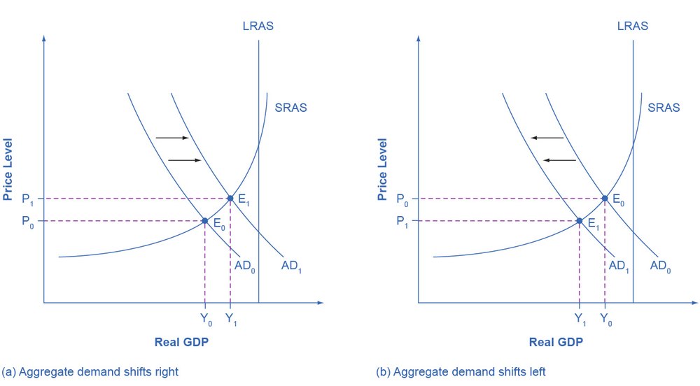
This is the labelling standard the FRQ expects: both curves named, both equilibria marked, and the price level and output read off each axis at each equilibrium.
Note that an economy can produce beyond Yf in the short run. It is not a physical ceiling: workers take overtime, plants run extra shifts. What makes it unsustainable is that it can only continue while wages lag prices, and wages eventually catch up.
Self-correction
Self-correction is an examinable mechanism, and the exam wants the chain, not the conclusion.
From a recessionary gap: high unemployment means workers compete for jobs → nominal wages fall (or rise more slowly) → firms' costs fall → SRAS shifts right → output returns to Yf at a lower price level.
From an inflationary gap: tight labour markets mean firms compete for workers → nominal wages are bid up → costs rise → SRAS shifts left → output returns to Yf at a higher price level.
Both end at Yf, because LRAS never moved. Demand-side changes cannot alter the long-run level of output, only where the economy sits relative to it, and at what price level.
**The policy debate is about speed.** Self-correction works, but nominal wages are famously slow to fall, workers resist cuts, and contracts are fixed for a year or more. So a recessionary gap can persist for a long time, which is the argument for intervening rather than waiting. Against that: intervention has lags of its own, and may arrive after correction has already happened.
Supply shocks
A negative supply shock, a sharp rise in oil prices, a natural disaster, a bad harvest, shifts SRAS left, raising the price level and cutting output. This is stagflation, and it is uniquely difficult because demand-side policy can address one problem only by worsening the other:
- Expansionary policy restores output but pushes the price level higher still.
- Contractionary policy brings inflation down but deepens the fall in output.
A positive supply shock shifts SRAS right, lowering the price level and raising output, the one case where both indicators improve at once.
When both curves shift
If AD and SRAS shift at the same time, one of the two outcomes becomes indeterminate, it depends on which shift is larger. This is a favourite multiple-choice construction, and the correct answer is often "indeterminate" or "cannot be determined".
| Price level | Real output | |
|---|---|---|
| AD right, SRAS right | Indeterminate | Rises |
| AD right, SRAS left | Rises | Indeterminate |
| AD left, SRAS right | Falls | Indeterminate |
| AD left, SRAS left | Indeterminate | Falls |
The pattern is worth seeing rather than memorising: when the two shifts push a variable the same way, it moves in that direction; when they push it in opposite directions; it is indeterminate.
The multipliers
An initial change in spending produces a larger final change in output, because one person's spending is another's income.
Define the leakages first:
- MPC = the fraction of extra income that is spent; MPS = the fraction saved. MPC + MPS = 1.
Spending multiplier = 1 ÷ (1 − MPC) = 1 ÷ MPS
Tax multiplier = −MPC ÷ (1 − MPC)
The tax multiplier is smaller in absolute value and negative. The reason is worth stating, because the exam asks for it: a tax cut raises disposable income, but households save part of it, so only MPC of the cut enters the spending stream in the first round. Government spending enters in full.
Balanced-budget multiplier = 1. Raising G and taxes by the same amount still raises output, because the spending multiplier exceeds the tax multiplier in absolute value. The net effect is exactly one times the change.
What reduces the multiplier: saving, taxation and imports all leak income out of the domestic spending stream. A more open or more heavily taxed economy has a smaller multiplier, which is a standard evaluation point when comparing the effectiveness of stimulus across countries.
A caution about the whole apparatus. The multiplier tells you how far AD shifts. It does not tell you how far real output rises, that depends on the slope of SRAS at the point the economy is sitting. Near Yf, most of a rightward AD shift becomes price level rather than output. Treating the multiplied figure as the increase in GDP is a common and costly slip.
Worked example
An economy is in short-run equilibrium below full employment. The government increases spending by \$50 billion, and MPC = 0.8.
Spending multiplier = 1 ÷ (1 − 0.8) = 5
Change in AD = 5 × \$50bn = \$250 billion
AD shifts right by the multiplied amount, \$250bn, not the initial \$50bn. That is a frequent lost point.
On the graph: AD shifts right; with output below Yf on an upward-sloping SRAS, real output rises and the price level rises, and unemployment falls towards the natural rate.
Compare a tax cut of the same size.
Tax multiplier = −0.8 ÷ 0.2 = −4, so a \$50bn tax cut raises AD by \$200bn.
The spending increase is more powerful, because the whole \$50bn is spent while only 80% of the tax cut is.
Now change the starting point. If the economy were already at Yf, the same stimulus would move it up the steep portion of SRAS: almost all of the effect would fall on the price level, with little output gain, demand-pull inflation. And in the long run, wages would adjust, SRAS would shift left, and output would return to Yf with the price level higher still.
Working backwards. The exam often reverses the question: an economy has a recessionary gap of \$300bn and MPC = 0.75. What spending increase closes it?
Spending multiplier = 1 ÷ 0.25 = 4
Required change in G = \$300bn ÷ 4 = \$75 billion
If the question asks for a tax change instead. Use the tax multiplier: −0.75 ÷ 0.25 = −3, so the required tax cut is \$300bn ÷ 3 = \$100 billion. The tax route always requires the larger number.
Common exam mistakes
- Explaining AD's slope with substitution between goods.
- Shifting AD by the initial injection rather than the multiplied amount.
- Using the spending multiplier for a tax change.
- Forgetting the tax multiplier is negative and smaller in magnitude.
- Reading the multiplied AD shift as the increase in real GDP, ignoring the slope of SRAS.
- Drawing LRAS as upward-sloping, in AP it is vertical at Yf.
- Shifting LRAS for a temporary supply shock, or for a change in AD.
- Counting transfer payments in G.
- Calling the purchase of shares "investment" in the AD sense.
- Labelling axes "price" and "quantity" instead of price level and real GDP.
- Claiming a rise in AD causes inflation without saying where the economy sits relative to Yf.
- Assuming both the price level and output move predictably when both curves shift.
Exam technique
Draw all three curves, AD, SRAS and LRAS, whenever the question involves the long run. Omitting LRAS makes it impossible to show an output gap, and the gap is usually where the points are.
Label axes Price Level and Real GDP (real output), mark Yf on the horizontal axis, and show the gap as the horizontal distance between equilibrium output and Yf. Label the new curve and new equilibrium too, examiners look for AD₁, AD₂, PL₁, PL₂, Y₁, Y₂ rather than an unlabelled second line.
Show multiplier working: formula, substitution, result, then the shift amount. Then state the effect on output, unemployment and the price level separately, each is typically its own point, and a sentence covering all three vaguely earns one mark instead of three.
For self-correction questions, name the variable that does the adjusting. The answer is nominal wages, and the curve that moves is SRAS. Answers that say "the economy returns to equilibrium" without that mechanism lose the bulk of the marks.
Quick revision
- AD = C + I + G + (X − M); slopes down via wealth, interest-rate and exchange-rate effects.
- G excludes transfer payments; I means capital spending by firms, not buying shares.
- SRAS slopes up because nominal wages are sticky; LRAS is vertical at Yf.
- Recessionary gap: output left of LRAS. Inflationary gap: right of it.
- Self-correction runs through nominal wage adjustment shifting SRAS, and always ends at Yf.
- Spending multiplier = 1 ÷ (1 − MPC); tax multiplier = −MPC ÷ (1 − MPC); balanced-budget = 1.
- Shift AD by the multiplied amount, but how much becomes output depends on the SRAS slope.
- Negative supply shock → SRAS left → stagflation.
- Both curves shifting → one variable is indeterminate.
Check you have it
Cross-board concept practice · originally a CIE 9708 question, used here because the concept is the same. It is not AP Economics past-paper material.
Question 1
According to Keynesian theory, what will cause the rate of interest to rise?
Answer: D.
Cross-board concept practice · originally a CIE 9708 question, used here because the concept is the same. It is not AP Economics past-paper material.
Question 2
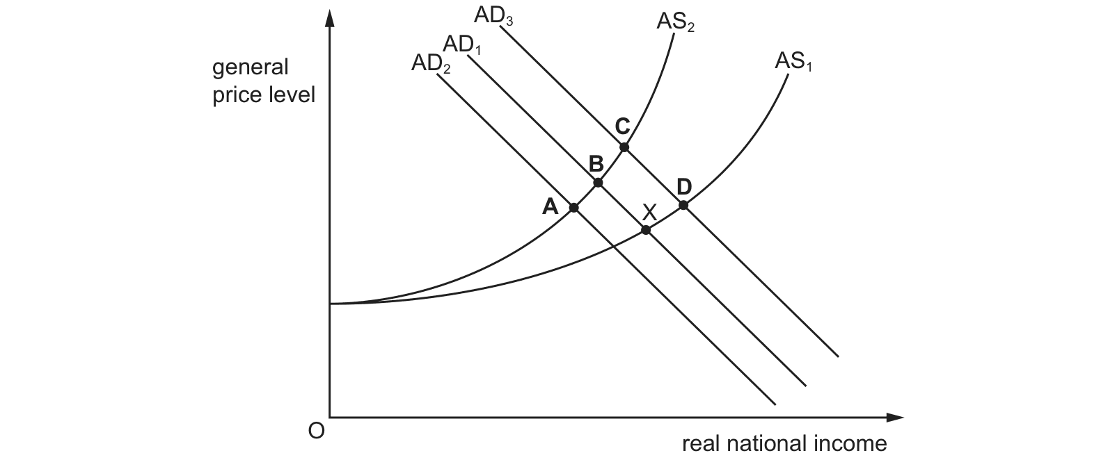
The aggregate demand (AD) and aggregate supply (AS) diagram shows an economy in equilibrium at X. In this economy, a severe shortage of raw materials causes a large rise in their price. The effect of this change is shown by a move to which point?
Answer: B.
Cross-board concept practice · originally a CIE 9708 question, used here because the concept is the same. It is not AP Economics past-paper material.
Question 3
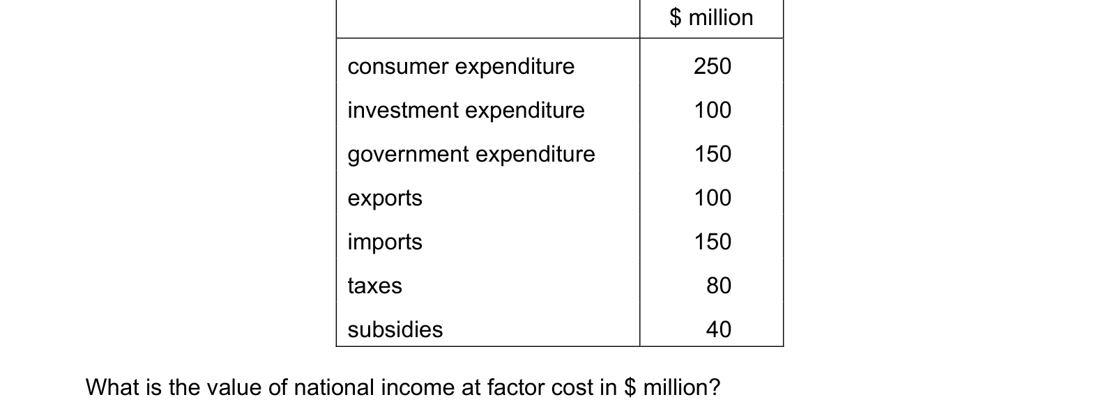
The information in the table is taken from a country’s national income accounts. $ million consumer expenditure 250 investment expenditure 100 government expenditure 150 exports 100 imports 150 taxes 80 subsidies 40 What is the value of national income at factor cost in $ million?
Answer: A.
What the syllabus asks for on this topicWhat this unit covers
What this unit covers
- Aggregate demand, its components and its determinants.
- Short-run and long-run aggregate supply, and why they differ.
- Macroeconomic equilibrium, output gaps and long-run self-correction.
- The spending, tax and balanced-budget multipliers.
- What happens when demand and supply shift at the same time.
At 17–27% of the multiple-choice section, this unit contains the model the rest of the course runs on. Units 4, 5 and 6 all end by shifting a curve on the AD–AS diagram, so a shaky grasp here costs marks in three other units as well as this one.
Related AP Economics topics
Not the topic you were looking for? Describe what you are stuck on in your own words and we will take you to the notes that answer it.