Production, Cost, and the Perfect Competition Model
Contents: 10 sections
Production and diminishing returns
The short run is the period in which at least one factor is fixed. The long run is when all factors are variable. These are defined by flexibility, not by clock time: the short run for a hairdresser may be weeks and for a power station a decade.
- Marginal product (MP) = the extra output from one more unit of labour.
- Average product (AP) = total output ÷ labour.
The law of diminishing marginal returns: as more of a variable factor is added to a fixed factor, marginal product eventually falls. Note eventually, MP often rises first, as early workers specialise and divide tasks. Diminishing returns set in because each additional worker has less of the fixed factor to work with.
This law is the origin of the cost curves, which is worth stating in a free-response answer:
- As MP falls, each additional unit of output requires more labour
- so marginal cost rises
- the MC curve slopes upward. Rising MC is the mirror image of falling MP.
MC and MP are inversely related, and MC cuts AVC and ATC at their minimum points. That is not a drawing convention: whenever marginal is below average, the average falls; when marginal is above, the average rises; so they cross exactly where the average is flat. The same arithmetic explains why MP cuts AP at AP's maximum.
Explicit costs, implicit costs and economic profit
This distinction underpins the whole unit's conclusion, and it is regularly examined in its own right.
- Explicit costs are payments actually made, wages, rent, materials.
- Implicit costs are the opportunity costs of resources the owner already owns, the salary forgone by running the business instead of taking a job, or the interest forgone on capital invested in it.
Accounting profit = total revenue − explicit costs
Economic profit = total revenue − explicit costs − implicit costs
Economic profit is therefore always lower than accounting profit, and it is the one economists mean. A firm earning zero economic profit is covering every explicit cost and matching what its owner's resources would have earned elsewhere. That is a perfectly satisfactory outcome; it is called normal profit, and it is why the long-run result below is not the disaster it sounds like.
Costs
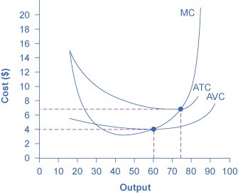
| Cost | Definition |
|---|---|
| Fixed cost (FC) | Does not vary with output; exists only in the short run |
| Variable cost (VC) | Varies with output |
| Total cost | TC = FC + VC |
| Average fixed cost | AFC = FC ÷ Q: always falling. Never U-shaped |
| Average variable cost | AVC = VC ÷ Q |
| Average total cost | ATC = TC ÷ Q = AFC + AVC |
| Marginal cost | MC = ΔTC ÷ ΔQ |
AFC falls continuously because a fixed amount is spread over more units, "spreading the overhead". This is why the gap between ATC and AVC narrows as output rises: that gap is AFC, and it shrinks towards zero without ever reaching it.
Note also that AVC reaches its minimum before ATC does. ATC is still being pulled down by falling AFC after AVC has begun to rise, so its turning point comes later and further right.
Fixed costs do not affect MC. Since fixed costs do not change with output, they drop out of ΔTC ÷ ΔQ entirely. A rise in rent shifts ATC up and leaves MC untouched, which means it does not change the profit-maximising quantity at all, only the profit earned there. AP tests this directly.
Long-run costs
In the long run, all costs are variable and the LRAC curve shows the lowest cost of producing each output when the firm can choose any scale:
- Economies of scale: LRAC falls as output rises (specialisation, bulk buying, spreading indivisible costs).
- Constant returns to scale: LRAC flat.
- Diseconomies of scale: LRAC rises (coordination and communication problems).
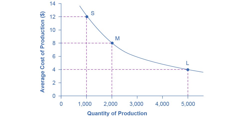
The figure shows the falling section only, average cost dropping from \$12 to \$4 as the scale of the plant rises. A complete LRAC curve for the exam should also show the flat and rising sections beyond this, giving the familiar U shape, with the lowest point marking the minimum efficient scale.
Distinguish diminishing returns (short run, one fixed factor, about marginal product) from diseconomies of scale (long run, all factors variable, about average cost). AP tests this confusion deliberately, and the giveaway is whether anything is being held fixed.
Profit maximisation
Every firm in every market structure maximises profit where:
MR = MC
The rule is marginal analysis again: while MR exceeds MC, the next unit adds more to revenue than to cost and is worth making; once MC exceeds MR; it is not.
For a perfectly competitive firm, the market price is given, so P = MR = AR, and the firm's demand curve is horizontal at the market price. That horizontal line is the single most distinctive feature of the model and the thing AP checks first. It follows from the firm being one seller among very many of an identical product: raise the price and buyers go elsewhere; there is no reason to lower it.
Profit per unit = P − ATC at the profit-maximising quantity. Total profit = (P − ATC) × Q, shown as a rectangle.
| Condition | Outcome |
|---|---|
| P > ATC | Economic profit |
| P = ATC | Break-even (normal profit) |
| AVC < P < ATC | Loss, but continue in the short run |
| P < AVC | Shut down |
The shut-down decision
The rule turns on AVC, not ATC, and the reasoning matters:
Fixed costs are paid whether or not the firm produces. So if price covers average variable cost, every unit sold contributes something towards fixed costs, and the loss is smaller than shutting down. Only when price falls below AVC does producing make the loss worse.
Put concretely: a firm with \$1,000 of fixed costs that shuts down loses \$1,000. If it can sell at a price covering its variable costs with anything left over, that surplus reduces the \$1,000 loss. It stays open not because it is profitable but because it is less unprofitable than closing.
The firm's short-run supply curve is therefore its MC curve above minimum AVC. Below that point, quantity supplied is zero. The market supply curve is the horizontal sum of every firm's.
In the long run there are no fixed costs, so the exit rule is simply P < ATC.
Perfect competition
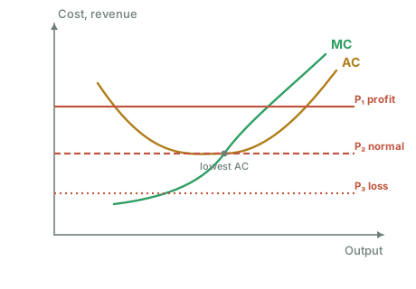
Assumptions: many buyers and sellers, an identical (homogeneous) product, perfect information, no barriers to entry or exit, and firms as price takers.
Short run: a firm can earn economic profit, break even, or make a loss, the three panels above.
Long run adjustment is the heart of the model:
- Economic profit attracts entry
- market supply increases
- market price falls
- firms' horizontal demand lines drop
- profit is competed away until P = minimum ATC, where economic profit is zero.
Losses drive the reverse: exit → supply decreases → price rises → back to zero economic profit.
Note what does the adjusting. The individual firm never chooses a price; it is the number of firms that changes, moving market supply and therefore the price every firm faces. Answers that have the firm cutting its price to compete have misunderstood the model.
At long-run equilibrium: P = MR = MC = minimum ATC. That single chain gives both efficiency results:
- Allocative efficiency: P = MC, so the value of the last unit to consumers equals its cost of production. Society produces exactly the quantity it values.
- Productive efficiency: production at minimum ATC, so no resources are wasted.
Zero economic profit does not mean firms earn nothing. It means they earn exactly what their resources could earn elsewhere, a normal return, and the implicit costs above are precisely what makes that true.
This double efficiency result is the benchmark the next unit measures monopoly against. Perfect competition is rare in reality; its role in the course is to be the standard of comparison.
Worked example
A competitive firm faces a market price of \$12. At its profit-maximising output of 500 units, ATC is \$10 and AVC is \$7.
Profit per unit = \$12 − \$10 = \$2 → total economic profit = \$2 × 500 = \$1,000.
Long run: that profit attracts entry, market supply shifts right, and price falls until it reaches minimum ATC. The firm ends earning zero economic profit, producing where P = MC = minimum ATC.
Change the price to \$8. Now P < ATC (\$10), so the firm makes a loss, but P > AVC (\$7), so each unit contributes \$1 towards fixed costs. It should continue producing in the short run and exit only if the price is still below ATC in the long run.
Loss at \$8 = (\$8 − \$10) × 500 = −\$1,000
Fixed costs = (ATC − AVC) × Q = (\$10 − \$7) × 500 = \$1,500
Shutting down would mean losing the whole \$1,500 of fixed costs. Producing loses only \$1,000. The firm is \$500 better off staying open, which is the shut-down rule in numbers.
Change the price to \$6. Now P < AVC (\$7). Every unit produced loses money before fixed costs are even considered, so the firm should shut down and lose only its \$1,500 of fixed costs.
Second worked example: building the cost table
A firm has fixed costs of \$50. Its output and variable costs are:
| Q | VC | TC | MC | AVC | ATC |
|---|---|---|---|---|---|
| 0 | \$0 | \$50 | : | : | : |
| 1 | \$30 | \$80 | \$30 | \$30 | \$80 |
| 2 | \$50 | \$100 | \$20 | \$25 | \$50 |
| 3 | \$80 | \$130 | \$30 | \$26.67 | \$43.33 |
| 4 | \$130 | \$180 | \$50 | \$32.50 | \$45 |
Read the structure off the table rather than memorising it:
- MC falls then rises: increasing returns first, then diminishing returns from the third unit.
- AVC is minimised at Q = 2 (\$25), and MC (\$20 → \$30) crosses AVC between units 2 and 3, exactly as the rule requires.
- ATC is minimised at Q = 3 (\$43.33), after AVC, because falling AFC is still pulling it down.
- ATC − AVC is \$43.33 − \$26.67 = \$16.67 at Q = 3, which is AFC = \$50 ÷ 3. The gap is always AFC.
If the market price were \$50, the firm would produce 4 units (where MC = \$50 = MR) and earn (\$50 − \$45) × 4 = \$20 of economic profit.
Common exam mistakes
- Drawing a downward-sloping demand curve for a perfectly competitive firm. It is horizontal.
- Using ATC instead of AVC for the shut-down decision.
- Saying zero economic profit means the firm makes no money.
- Ignoring implicit costs, and so reporting accounting profit as economic profit.
- Confusing diminishing returns (short run) with diseconomies of scale (long run).
- Drawing MC cutting ATC anywhere other than its minimum.
- Drawing AFC as U-shaped, it falls continuously.
- Putting AVC's minimum at the same output as ATC's. AVC turns first.
- Letting a change in fixed cost move the MC curve or the profit-maximising quantity.
- Having the individual firm cut its price to compete, rather than entry shifting market supply.
Exam technique
Draw the side-by-side market and firm graphs, and line the price up at the same height on both. Readers expect this layout and check that the firm's horizontal demand line matches the market price.
Mark quantity where MR = MC, then shade profit or loss as a rectangle between price and ATC. Label it, an unlabelled rectangle is not credited.
When asked about the long run, describe the mechanism, entry, supply shift, price fall, not just the end state. The marks are in the adjustment process, and "profit falls to zero" on its own earns almost nothing.
If a question gives you a cost table, compute MC as the change in total cost between rows, not as a total divided by anything. It is the single most common table error.
Quick revision
- Diminishing marginal returns cause MC to rise; MC cuts AVC and ATC at their minimums.
- AFC always falls; ATC = AFC + AVC; the ATC–AVC gap is AFC.
- AVC bottoms out before ATC does.
- Fixed costs do not affect MC, so they never change the optimal quantity.
- Economic profit subtracts implicit costs too; zero economic profit = normal profit.
- Diminishing returns = short run, marginal product. Diseconomies = long run, average cost.
- All firms maximise profit at MR = MC; for perfect competition P = MR = AR.
- Shut down if P < AVC; the short-run supply curve is MC above minimum AVC.
- Long run: entry or exit drives economic profit to zero at P = minimum ATC.
- Perfect competition achieves both allocative (P = MC) and productive (min ATC) efficiency.
Check you have it
Cross-board concept practice · originally a CIE 9708 question, used here because the concept is the same. It is not AP Economics past-paper material.
Question 1
What is likely to facilitate the growth of large firms in an economy?
Answer: B.
Explanation:
The correct answer is B - dividend payments are a low proportion of company profits.
Large firms are more likely to grow in an economy when dividend payments are a low proportion of company profits. When companies retain a higher proportion of their profits rather than paying them out as dividends, they have more funds available for reinvestment in business expansion, research and development, new technologies, mergers, acquisitions, and other growth opportunities. This behaviour enables large firms to scale their operations, enter new markets, and increase their competitive advantage.
Options A, C, and D are unlikely to facilitate the growth of large firms:
A - an industry structure which approximates to perfect competition: In a perfectly competitive market, firms are price takers, and there are many small firms. Large firms may struggle to grow in such an environment due to intense competition and limited market power.
C - government regulations preventing takeovers: Regulations preventing takeovers can limit the ability of firms to grow through acquisitions and mergers, which are common strategies for large firms to expand their market presence and achieve economies of scale.
D - the existence of managerial diseconomies of scale: Managerial diseconomies of scale occur when the efficiency of management decreases as a firm grows larger. This can hinder the growth of large firms as inefficiencies may increase with size, making it challenging to manage and operate the business effectively.
Therefore, among the given options, B is the most likely factor to facilitate the growth of large firms in an economy.
Cross-board concept practice · originally a CIE 9708 question, used here because the concept is the same. It is not AP Economics past-paper material.
Question 2
A firm has very high fixed costs but low marginal costs of production. It experiences continuous economies of scale so that the minimum efficient scale is not reached until the firm is very large in relation to total market demand.
In which type of market structure would the firm operate?
Answer: C.
Every detail in the question points to it. Very high fixed costs with low marginal costs mean average cost falls steadily as output grows, since the large fixed cost is spread over more and more units. Continuous economies of scale with a minimum efficient scale that is very large relative to total market demand means the market is only big enough for one firm to reach the lowest point on its average cost curve. A second firm entering would leave both producing at higher average cost than one firm alone. Water supply, electricity transmission and rail infrastructure fit this pattern, which is why they are typically single suppliers subject to regulation.
Why the other options are wrong:
- A, monopolistic competition, has many small firms with differentiated products and low barriers to entry. Extensive economies of scale relative to market size make many firms impossible.
- B, monopsony, describes a single buyer rather than a single seller. The question describes a producer's cost structure, which says nothing about buying power.
- D, oligopoly, has a few large firms sharing the market. If minimum efficient scale is not reached until a firm is very large relative to total demand, the market cannot sustain several firms at efficient scale.
Cross-board concept practice · originally a CIE 9708 question, used here because the concept is the same. It is not AP Economics past-paper material.
Question 3
A firm in monopolistic competition that is producing at its profit maximising output is making a loss in the short run. For it to continue in production, what must be correct about its average revenue (AR), marginal revenue (MR) and average variable cost (AVC)?
Answer: D.
What the syllabus asks for on this topicWhat this unit covers
What this unit covers
- The production function, marginal product and diminishing returns.
- Explicit and implicit costs, and the difference between accounting and economic profit.
- Short-run and long-run costs.
- Profit maximisation and the shut-down decision.
- Perfect competition in the short run and long run.
This unit builds the cost apparatus that Units 4 and 5 then reuse without reintroducing. A monopoly diagram is a perfect-competition diagram with a different demand curve, so every cost curve learned here reappears there, and errors made here are repeated three more times.
Related AP Economics topics
Not the topic you were looking for? Describe what you are stuck on in your own words and we will take you to the notes that answer it.