Imperfect Competition
Contents: 9 sections
Why imperfect competition differs
Every firm maximises profit where MR = MC. What changes across market structures is the demand curve the firm faces.
A perfectly competitive firm is a price taker with a horizontal demand curve, so P = MR. Every imperfectly competitive firm faces a downward-sloping demand curve, which means selling one more unit requires lowering the price, and for a single-price firm, lowering it on every unit.
Therefore MR < P for any firm with market power. Profit maximisation at MR = MC then gives an output where P > MC, which is the source of allocative inefficiency in this whole unit.
The arithmetic is worth seeing once. Suppose a firm sells 3 units at \$10 (revenue \$30) and must cut the price to \$9 to sell a fourth (revenue \$36). Marginal revenue is \$6, not \$9: the firm gained \$9 on the new unit but lost \$1 on each of the three it could have sold at \$10. That loss on the earlier units is exactly why MR falls below price.
For a straight-line demand curve, MR is twice as steep and lies below demand, hitting the horizontal axis halfway to where demand does. Drawing MR on top of demand is the most common error in AP Micro.
The four market structures
| Perfect competition | Monopolistic competition | Oligopoly | Monopoly | |
|---|---|---|---|---|
| Number of firms | Very many | Many | Few | One |
| Product | Identical | Differentiated | Either | Unique |
| Barriers to entry | None | Low | High | Very high |
| Firm's demand | Horizontal | Downward, elastic | Downward | Downward, market demand |
| P vs MC | P = MC | P > MC | P > MC | P > MC |
| Long-run profit | Zero | Zero | Can persist | Can persist |
| Allocatively efficient? | Yes | No | No | No |
| Productively efficient? | Yes | No (excess capacity) | No | No |
Only the first column achieves either efficiency. Everything else in this unit is a variation on how and why firms depart from it.
Monopoly
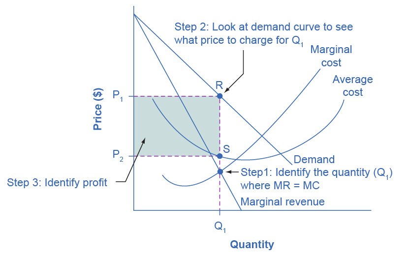
A single seller, a unique product, and high barriers to entry, economies of scale, control of a resource, patents, or legal protection.
Finding price and quantity:
- Locate quantity where MR = MC.
- Read up to the demand curve for price. Never read price off MR.
Outcomes: output is lower and price higher than under perfect competition. There is deadweight loss, shown as the triangle between demand and MC, from the monopoly quantity out to the allocatively efficient quantity where P = MC.
Efficiency: a monopoly is allocatively inefficient (P > MC) and typically productively inefficient too (it does not produce at minimum ATC). Because barriers block entry, economic profit can persist in the long run.
A monopoly is not guaranteed a profit. If demand is weak relative to costs, ATC lying above the demand curve at every output, the monopolist makes a loss and will exit in the long run. Market power means control over price, not a promise of profit, and AP asks this to check the distinction.
Monopolies never operate on the inelastic portion of demand. Where demand is inelastic, MR is negative, and no firm maximises profit where marginal revenue is below zero while marginal cost is positive. The profit-maximising point always lies on the elastic half.
Natural monopoly: where economies of scale are so large that ATC falls across the whole relevant range, one firm supplies more cheaply than several. Regulation options:
- Socially optimal price (P = MC): allocatively efficient, but with ATC above MC throughout, the firm makes a loss and needs a subsidy to survive.
- Fair-return price (P = ATC): the firm breaks even with zero economic profit, but output remains below the allocatively efficient level.
That trade-off is a standard FRQ, and naming both prices with their consequences is what earns the points.
Price discrimination
Charging different prices to different buyers for the same good, where the price difference does not reflect cost.
Three conditions must hold: market power, the ability to segment buyers by willingness to pay, and the ability to prevent resale between segments.
Under perfect (first-degree) price discrimination, the firm charges each buyer their maximum willingness to pay. The results are distinctive and heavily tested:
- The demand curve becomes the MR curve, since no price cut on earlier units is needed.
- Output rises to the allocatively efficient level where P = MC.
- Deadweight loss is zero.
- All consumer surplus is captured as producer surplus.
So perfect price discrimination is efficient but highly inequitable, the efficiency gain goes entirely to the firm. This is the cleanest example in the course of efficiency and equity pointing in opposite directions.
In practice firms discriminate imperfectly, charging different prices to identifiable groups, student and senior discounts, peak and off-peak fares, business and leisure air fares. The group charged the higher price is the one with the more inelastic demand.
Monopolistic competition
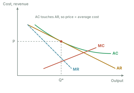
Many firms, differentiated products, and low barriers to entry.
Each firm faces a downward-sloping but relatively elastic demand curve, because close substitutes exist. Differentiation may be real (quality, features) or perceived (branding, advertising), either gives the firm some power over its own price.
Short run: economic profit or loss is possible, exactly as in monopoly, the figure above shows the profit case.
Long run: low barriers mean entry competes profit away. Entry shifts each existing firm's demand curve left (and makes it more elastic) until demand is tangent to ATC.
At long-run equilibrium:
- Zero economic profit (P = ATC at the tangency).
- P > MC, so still allocatively inefficient.
- Production is not at minimum ATC, so productively inefficient, the gap between actual output and minimum-ATC output is called excess capacity.
The trade-off worth stating: consumers pay above marginal cost and firms operate below efficient scale, but in exchange get product variety. Whether that is worth it is a genuine judgement, and an FRQ asking you to evaluate monopolistic competition wants both halves.
Oligopoly and game theory
A few large interdependent firms. Interdependence is the defining feature: each firm's best action depends on what rivals do, which is why oligopoly needs game theory rather than a single diagram.
Game theory analyses this with a payoff matrix. Two ideas AP tests directly:
- Dominant strategy: a strategy that is best for a player regardless of what the other does. A player may have one, both players may, or neither may.
- Nash equilibrium: a cell where neither player can improve by unilaterally changing strategy, given the other's choice.
Read a matrix one player at a time: fix the opponent's choice, compare that player's payoffs, and underline the better one. Where both players' best responses coincide, that cell is a Nash equilibrium.
Reading a payoff matrix
Two firms each choose a high or low price. Each cell shows (Firm A's profit, Firm B's profit) in millions:
| B: High price | B: Low price | |
|---|---|---|
| A: High price | (10, 10) | (2, 15) |
| A: Low price | (15, 2) | (5, 5) |
Firm A's reasoning, holding B's choice fixed each time:
- If B prices high, A earns 10 by pricing high and 15 by pricing low
- low is better.
- If B prices low, A earns 2 by pricing high and 5 by pricing low
- low is better.
Low is better in both cases, so pricing low is A's dominant strategy. The matrix is symmetric, so the same holds for B.
The Nash equilibrium is (Low, Low), paying (5, 5). Neither firm can improve by changing on its own: from (5,5), A switching to high would drop it to 2.
Notice the outcome. Both firms would earn 10 if both priced high, better for both than the 5 they actually get. That is the prisoner's dilemma structure, and it is the standard exam conclusion: individually rational choices produce a jointly worse result.
Collusion would let the firms reach the (10, 10) cell, which is why cartels form. But each firm still has an incentive to cheat by undercutting, from (10,10), defecting raises that firm's payoff to 15. That incentive is why cartels are unstable even before considering that they are usually illegal.
The dilemma is weaker when the game is repeated, because a firm that cheats can be punished by rivals in later rounds. Sustained collusion is more likely among few firms, with easily observed prices and repeated interaction.
Worked example
A monopolist faces demand P = 100 − 2Q and constant MC = 20.
Total revenue = P × Q = 100Q − 2Q² → MR = 100 − 4Q (twice as steep as demand).
Set MR = MC: 100 − 4Q = 20 → Q = 20.
Price: read up to demand, not MR → P = 100 − 2(20) = \$60.
Compare with perfect competition, where P = MC: 100 − 2Q = 20 → Q = 40 at a price of \$20.
So the monopoly produces half the competitive output at three times the price. Deadweight loss is the triangle between demand and MC from Q = 20 to Q = 40: ½ × (60 − 20) × (40 − 20) = \$400.
Now make the same firm a perfect price discriminator. It charges each buyer their willingness to pay, so demand becomes MR, and it produces where demand meets MC, Q = 40, the competitive quantity. Deadweight loss falls to zero, and the entire consumer surplus, ½ × (100 − 20) × 40 = \$1,600, is captured by the firm as producer surplus. Output rose, efficiency was restored, and consumers were left with nothing.
Common exam mistakes
- Drawing MR on top of, or above, the demand curve.
- Reading the monopoly price off the MR curve instead of up to demand.
- Assuming a monopoly must earn a profit.
- Putting the monopoly's output on the inelastic portion of demand.
- Claiming monopolistic competition earns long-run economic profit, entry removes it.
- Forgetting excess capacity in monopolistic competition.
- Drawing long-run monopolistic competition with demand crossing ATC rather than tangent to it.
- Saying price discrimination always harms consumers, total output actually rises.
- Confusing a dominant strategy with a Nash equilibrium. A dominant strategy belongs to one player; a Nash equilibrium is a cell.
- Omitting resale prevention from the conditions for price discrimination.
Exam technique
Draw demand, MR (below and twice as steep), MC and ATC. Mark quantity at MR = MC, take price up to demand, shade profit between price and ATC, and shade deadweight loss between demand and MC out to where P = MC. Label every area, readers credit labelled areas, not shapes they must interpret.
For monopolistic competition in the long run, the defining feature is demand tangent to ATC. Draw the tangency deliberately, because a reader checks for it. A demand curve that cuts through ATC implies profit or loss and contradicts your own answer.
For game theory, work through the matrix explicitly, stating each player's best response given each choice of the other before naming the equilibrium. Writing "Low is dominant for A because 15 > 10 and 5 > 2" shows the reasoning the rubric asks for.
Quick revision
- Downward-sloping demand → MR < P → profit maximisation gives P > MC.
- MR is twice as steep as a linear demand curve.
- Monopoly: Q where MR = MC, P read up to demand; DWL between demand and MC.
- A monopoly can still make a loss, and never produces where demand is inelastic.
- Natural monopoly: P = MC is efficient but loss-making; P = ATC breaks even.
- Price discrimination needs market power, segmentation and no resale; perfect discrimination gives zero DWL and no consumer surplus.
- Monopolistic competition: long-run zero profit, demand tangent to ATC, excess capacity, P > MC.
- Dominant strategy = best regardless of the rival. Nash = neither wants to deviate.
- The prisoner's dilemma: both firms defect and both end worse off than under collusion.
Check you have it
Cross-board concept practice · originally a CIE 9708 question, used here because the concept is the same. It is not AP Economics past-paper material.
Question 1
The diagram shows a firm in imperfect competition. It changed its aim from profit maximising to sales revenue maximising. Which type of profit was it making in each case?
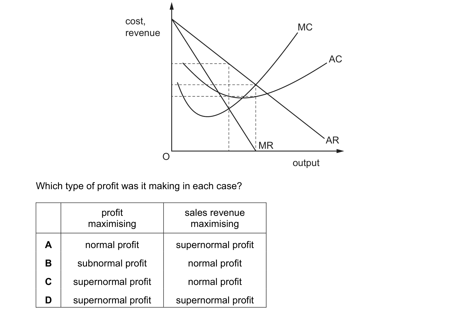
Answer: D.
Cross-board concept practice · originally a CIE 9708 question, used here because the concept is the same. It is not AP Economics past-paper material.
Question 2
For a firm in imperfect competition, the marginal revenue product of labour at any given level of employment is equal to
Answer: C.
What the syllabus asks for on this topicWhat this unit covers
What this unit covers
- Monopoly: price, output, efficiency and regulation.
- Price discrimination.
- Monopolistic competition in the short and long run.
- Oligopoly and game theory.
Related AP Economics topics
Not the topic you were looking for? Describe what you are stuck on in your own words and we will take you to the notes that answer it.