Factor Markets
Contents: 9 sections
Derived demand
Demand for a factor of production is derived demand: firms want labour not for itself but for the output it produces. So when demand for the product rises, demand for the labour that makes it rises too.
This has a consequence worth carrying into every answer in this unit: anything that changes the product market changes the factor market. A fall in the price of the finished good reduces labour demand even though nothing about the workers has changed.
This unit has no close counterpart in most non-US syllabuses, and it is where borrowed practice material runs out, the marginal revenue product framework is specifically how AP builds labour demand.
Marginal revenue product
MRP is the extra revenue from hiring one more unit of a factor.
MRP = MP × MR
For a firm selling in a perfectly competitive product market, MR equals price, so this simplifies to MRP = MP × P (sometimes called the value of the marginal product).
For a firm with market power in the product market, MR is below price and falls as output rises. MRP therefore falls for two reasons at once, diminishing marginal product and falling marginal revenue, so the MRP curve is steeper. AP asks about this distinction directly, and the consequence is that a firm with product-market power hires fewer workers than a competitive firm facing the same technology.
MRP slopes downward because of diminishing marginal returns: each additional worker adds less output than the last.
The hiring rule
MRC (marginal resource cost, or marginal factor cost) is the extra cost of hiring one more unit.
Hire while MRP > MRC, and stop where MRP = MRC.
This is the same MB = MC logic as everywhere else in the course, applied to inputs.
Least-cost combination of two inputs, the cost-minimising rule:
MP₍L₎ ÷ P₍L₎ = MP₍K₎ ÷ P₍K₎
The intuition: if a dollar spent on labour buys more extra output than a dollar spent on capital, the firm should shift spending towards labour. Only when the last dollar spent on each input yields the same extra output is there nothing left to gain by reallocating.
Profit-maximising combination, a stronger condition, requiring each input to pay for itself:
MRP₍L₎ ÷ P₍L₎ = MRP₍K₎ ÷ P₍K₎ = 1
A firm can be at least-cost without maximising profit; the ratio equalling 1 is what adds the profit condition. Producing the wrong quantity as cheaply as possible still satisfies the first rule and fails the second.
Perfectly competitive labour markets
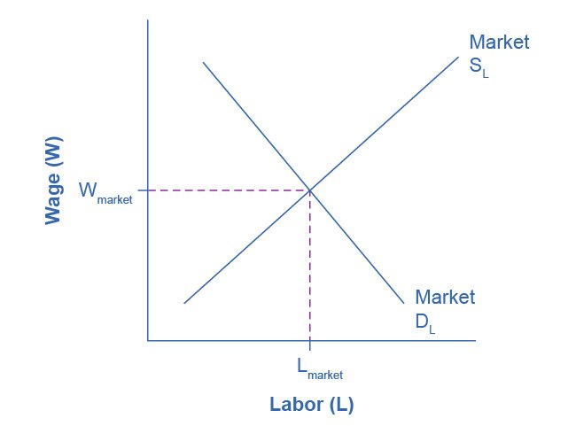
Many small firms and many workers, with an identical type of labour and no wage-setting power. The firm is a wage taker.
Draw this as side-by-side graphs, exactly as in Unit 3:
- Market graph: upward-sloping labour supply, downward-sloping labour demand (the sum of firms' MRP curves), setting the equilibrium wage.
- Firm graph: a horizontal labour supply curve at that wage, so wage = MRC, plus the firm's downward-sloping MRP curve.
The firm hires where MRP = wage.
What shifts each curve
Shifters of labour demand:
- Product demand: a rise in demand for the output raises MR and shifts MRP right. This is derived demand at work.
- Productivity: better training, technology or capital raises MP and shifts MRP right.
- The price of other inputs: and the direction depends on the relationship. If capital is a substitute for labour, cheaper capital shifts labour demand left. If capital is a complement, cheaper capital raises the productivity of labour and shifts demand right. Deciding which relationship applies is the whole question.
Shifters of labour supply: the number of qualified workers, immigration, the wages available in alternative occupations, non-wage benefits and working conditions, and training or licensing requirements. Anything that raises the cost of entering an occupation reduces its supply and raises its equilibrium wage, which is a large part of why wages differ across occupations at all.
Monopsony
A single buyer of labour, a company town, or a specialised employer.
The monopsonist faces the upward-sloping market labour supply curve, which means hiring one more worker requires raising the wage. If it must pay that higher wage to every worker already employed, the cost of an additional worker exceeds that worker's wage.
Therefore MRC lies above the labour supply curve, and is steeper.
This is the exact mirror image of monopoly, where MR lies below demand, and the procedure mirrors it too:
- Find quantity of labour where MRC = MRP.
- Read the wage down to the labour supply curve. Never off MRC.
Outcome: the monopsonist hires fewer workers at a lower wage than a competitive labour market would produce. Both employment and wages are below the competitive level.
A minimum wage in a monopsony can therefore raise both the wage and employment, up to the competitive level, the opposite of its effect in a competitive labour market, where a binding minimum wage causes unemployment. This counter-intuitive result is a favourite AP question, and it depends entirely on identifying the market structure first.
The reason it works is worth stating: a minimum wage removes the monopsonist's incentive to hold employment down. Once the wage is fixed by law, hiring an extra worker no longer forces a raise for everyone else, so MRC becomes flat at the minimum wage, and the firm hires until MRP meets it, exactly as a competitive firm would.
Worked example
A firm's MRP schedule, with the firm hiring in a competitive labour market at a wage of \$18 per hour:
| Workers | Total output | MP | MRP (at P = \$5) |
|---|---|---|---|
| 1 | 7 | 7 | \$35 |
| 2 | 13 | 6 | \$30 |
| 3 | 18 | 5 | \$25 |
| 4 | 22 | 4 | \$20 |
| 5 | 25 | 3 | \$15 |
Hire while MRP ≥ wage. The fourth worker's MRP is \$20 ≥ \$18, so hire. The fifth worker's MRP is \$15 < \$18, so do not.
The firm employs 4 workers.
Second worked example: monopsony in numbers
The same MRP schedule, but now the firm is the only employer and must raise the wage to attract each additional worker:
| Workers | Wage | Total labour cost | MRC | MRP |
|---|---|---|---|---|
| 1 | \$10 | \$10 | \$10 | \$35 |
| 2 | \$12 | \$24 | \$14 | \$30 |
| 3 | \$14 | \$42 | \$18 | \$25 |
| 4 | \$16 | \$64 | \$22 | \$20 |
| 5 | \$18 | \$90 | \$26 | \$15 |
MRC is the change in total labour cost, not the wage. Hiring the third worker costs \$18: \$14 for that worker, plus the \$2 raise given to each of the two already employed.
Hire while MRP ≥ MRC. Third worker: MRP \$25 ≥ MRC \$18 → hire. Fourth worker: MRP \$20 < MRC \$22 → do not.
The monopsonist employs 3 workers and pays the wage read down to supply: \$14.
Compare the competitive outcome with the same supply schedule, where each firm takes the wage as given and hires while MRP ≥ wage. At 4 workers the wage is \$16 and MRP is \$20, so the fourth is hired; at 5 the wage is \$18 and MRP \$15, so the fifth is not. Competition gives 4 workers at \$16.
So the monopsonist employs one fewer worker and pays \$2 less, exactly as the theory predicts.
Now impose a minimum wage of \$16. The firm must pay \$16 regardless of how many it hires, so MRC is flat at \$16 up to 4 workers, hiring one more no longer means raising everyone's pay.
Hire while MRP ≥ \$16. Fourth worker: MRP \$20 ≥ \$16 → hire. Fifth: MRP \$15 < \$16 → do not.
Employment rises to 4 and the wage rises to \$16.
Both went up. That is the result AP wants, and it is only possible because the market was monopsonistic to begin with.
Common exam mistakes
- Using MP instead of MRP in the hiring rule.
- Forgetting that MRP = MP × MR, and that MR = P only in a competitive product market.
- Computing MRC as the wage rather than as the change in total labour cost.
- Drawing MRC below the labour supply curve in monopsony, it lies above.
- Reading the monopsony wage off the MRC curve instead of down to supply.
- Claiming a minimum wage always causes unemployment, without checking whether the market is monopsonistic.
- Confusing the least-cost rule (MP/P equal) with the profit-maximising rule (MRP/P = 1).
- Treating labour demand as if it were independent of product demand.
- Assuming cheaper capital always reduces labour demand, it depends on whether capital substitutes for or complements labour.
Exam technique
Label axes Wage and Quantity of Labour, not price and quantity. Readers check.
Use the side-by-side market and firm layout for competitive labour markets, with the firm's labour supply horizontal at the market wage.
For monopsony, draw one graph with labour supply, MRC above it, and MRP. Mark the quantity at MRC = MRP with a dotted line, then take the wage down to supply and label it clearly, the two-step read is where the points are, and it is the same two-step read as the monopoly diagram in Unit 4.
Show calculations in a table when given data. MRP per worker is easier to compare against MRC in tabular form, and the table itself usually earns credit.
Quick revision
- Factor demand is derived from product demand.
- MRP = MP × MR; MR = P only in a competitive product market.
- Hire where MRP = MRC; least cost when MP/P is equal across inputs; profit maximised when MRP/P = 1.
- Competitive labour market: firm is a wage taker, labour supply to the firm is horizontal, wage = MRC.
- Monopsony: MRC above supply; quantity at MRC = MRP; wage read down to supply.
- MRC is the change in total labour cost, which exceeds the wage because everyone gets the raise.
- Monopsony gives lower wages and lower employment than competition.
- A minimum wage can raise both wages and employment under monopsony, because it flattens MRC.
Check you have it
Cross-board concept practice · originally a CIE 9708 question, used here because the concept is the same. It is not AP Economics past-paper material.
Question 1
An increase in the world price of oil increases the demand for deep sea divers from D to D as 1 2 shown. V S wage Y W X T R D Q D 1 2 O M N number of divers What is the change in the economic rent earned by the divers?
Answer: C.
Cross-board concept practice · originally a CIE 9708 question, used here because the concept is the same. It is not AP Economics past-paper material.
Question 2
What happens to economic rent and transfer earnings if the supply of labour becomes perfectly inelastic?
Answer: C.
Cross-board concept practice · originally a CIE 9708 question, used here because the concept is the same. It is not AP Economics past-paper material.
Question 3
What represents the transfer earnings of the factor enterprise?
Answer: B.
What the syllabus asks for on this topicWhat this unit covers
What this unit covers
- Derived demand and marginal revenue product.
- Perfectly competitive labour markets.
- Shifts in factor demand and factor supply.
- Monopsony and imperfect factor markets.
- The least-cost and profit-maximising rules for hiring inputs.
Related AP Economics topics
Not the topic you were looking for? Describe what you are stuck on in your own words and we will take you to the notes that answer it.