Supply and Demand
Contents: 9 sections
Demand and supply
Demand slopes downward because of the substitution and income effects: a lower price makes the good cheaper relative to alternatives, and raises real purchasing power.
Supply slopes upward because higher prices cover rising marginal costs, and because production becomes profitable for more firms.
Distinguish a change in quantity demanded (a movement along the curve, caused only by the good's own price) from a change in demand (a shift, caused by anything else). AP marks these as different things, and using the wrong phrase costs the point.
Demand shifters: income, prices of substitutes and complements, tastes, expectations, number of buyers. Supply shifters: input prices, technology, taxes and subsidies, expectations, number of sellers.
For income, the direction depends on the good: higher income raises demand for a normal good and lowers it for an inferior good.
For related goods, be precise about which curve moves. A rise in the price of a substitute raises demand for this good; a rise in the price of a complement lowers it. Note that both act on demand, a change in the price of a related good never shifts this good's supply.
Expectations cut both ways and are worth thinking through rather than memorising. If consumers expect a price rise, they buy now: demand rises today. If producers expect a price rise, they withhold stock: supply falls today.
Market equilibrium
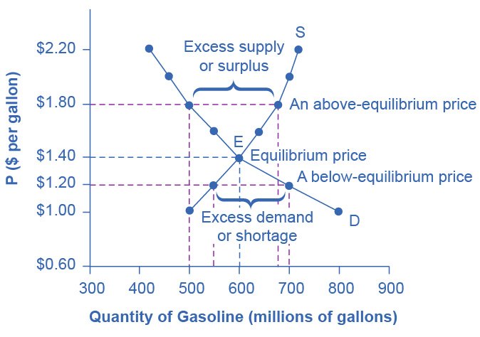
Equilibrium is where quantity demanded equals quantity supplied. Above it there is a surplus, pushing price down; below it a shortage, pushing price up. Both correct through movements along the curves, not shifts.
When both curves shift, one outcome is determinate and the other is ambiguous:
| Price | Quantity | |
|---|---|---|
| D right, S right | Indeterminate | Rises |
| D right, S left | Rises | Indeterminate |
| D left, S right | Falls | Indeterminate |
| D left, S left | Indeterminate | Falls |
The pattern rather than the table: when both shifts push a variable the same way it moves that way; when they push in opposite directions it is indeterminate. AP asks this explicitly, and the correct answer is "indeterminate" with a reason, not a guess.
Elasticity
Elasticity measures responsiveness: how much one variable changes in percentage terms when another does.
| Measure | Formula | Reading |
|---|---|---|
| PED | %ΔQd ÷ %ΔP | >1 elastic, <1 inelastic (use absolute value) |
| PES | %ΔQs ÷ %ΔP | >1 elastic, <1 inelastic |
| YED | %ΔQd ÷ %ΔIncome | + normal, − inferior |
| XED | %ΔQd of A ÷ %ΔP of B | + substitutes, − complements |
The two income-related measures are where sign matters most. A negative YED identifies an inferior good, and a YED above 1 identifies a luxury, whose demand grows faster than income. A negative XED identifies complements, because the two goods move in opposite directions; a positive XED identifies substitutes. Reading the sign is usually the whole question.
Total revenue test: if demand is elastic, a price rise lowers total revenue; if inelastic, a price rise raises it. At unit elasticity, revenue is unchanged and at its maximum.
The logic is worth holding rather than memorising: total revenue is price × quantity, so a price rise pulls revenue up and the resulting fall in quantity pulls it down. Whichever effect is proportionally larger wins, and elasticity is precisely the measure of which that is.
Determinants of PED: availability of substitutes (much the strongest), the share of income the good absorbs, whether it is a necessity or a luxury, and time, demand is more elastic over longer horizons, because buyers need time to find alternatives.
Determinants of PES: the availability of spare capacity, how easily inputs can be obtained, whether the good can be stored, and again time. Supply is almost always more elastic in the long run, when firms can build capacity and new firms can enter.
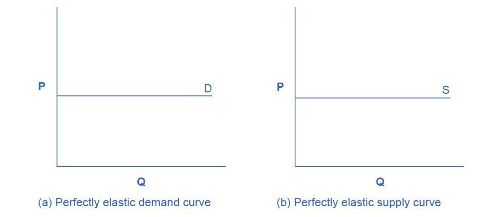
The extreme cases are worth recognising on sight, because AP uses them to make incidence questions unambiguous:
- Perfectly elastic (horizontal, PED = ∞), any price rise loses every buyer.
- Perfectly inelastic (vertical, PED = 0), quantity does not respond to price at all.
PED varies along a straight-line demand curve: elastic on the upper section, unit elastic at the midpoint, inelastic on the lower section. This follows from PED being a ratio of percentage changes with shifting base values, and AP has tested it directly. It is also why "the demand for this good is inelastic" is an incomplete statement unless you say where on the curve.
The midpoint formula avoids the problem that percentage changes differ depending on direction:
% change = (new − old) ÷ [(new + old) ÷ 2] × 100
Surplus and welfare
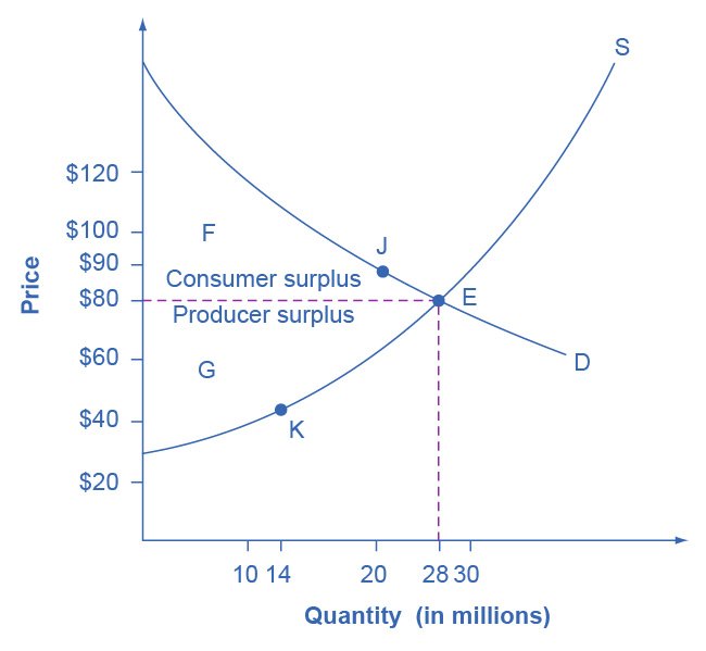
- Consumer surplus: the area below the demand curve and above the price, what buyers were willing to pay, minus what they did pay.
- Producer surplus: the area above the supply curve and below the price, what sellers received, minus the minimum they would have accepted.
- At competitive equilibrium, total surplus is maximised, the market is allocatively efficient, and price equals marginal cost.
The reason equilibrium maximises surplus is worth being able to state. Every unit up to equilibrium has a value to some buyer above its cost to some seller, so trading it creates surplus. Past equilibrium, cost exceeds value, so trading it would destroy surplus. The equilibrium quantity is exactly the point where those run out.
Any deviation from equilibrium creates deadweight loss: the triangle of surplus destroyed because mutually beneficial trades no longer happen. Since these areas are triangles, the arithmetic is nearly always ½ × base × height, and identifying which distance is which is most of the work.
Government intervention
Price controls
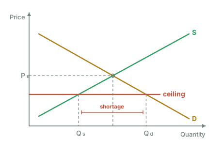
- A binding price ceiling sits below equilibrium and creates a shortage.
- A binding price floor sits above equilibrium and creates a surplus.
- A ceiling above equilibrium, or a floor below it, is non-binding and changes nothing. AP frequently offers a non-binding control to see whether you check.
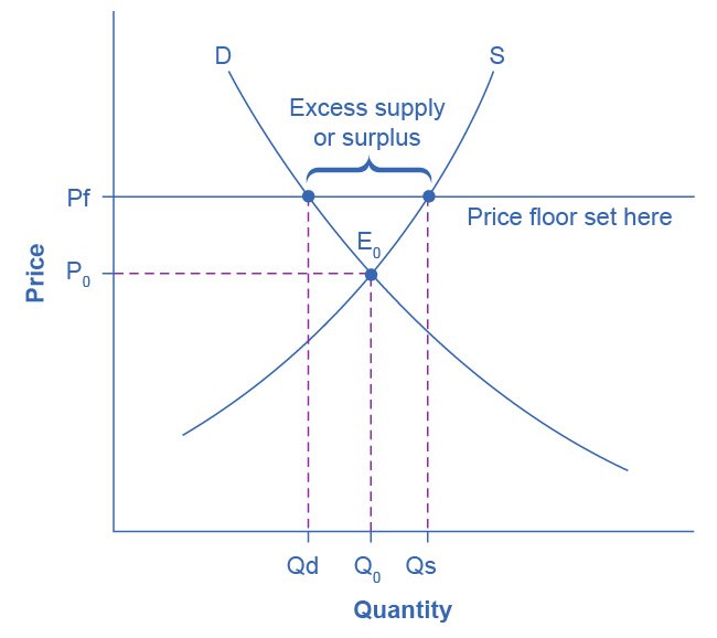
Both controls destroy surplus, because both cut the quantity traded below equilibrium. Note that this is the key insight: a ceiling reduces quantity because less is supplied, while a floor reduces quantity because less is demanded, but either way the quantity actually traded falls, and deadweight loss follows.
The consequences beyond the diagram are standard evaluation material. A binding ceiling produces queues, rationing, falling quality as sellers economise, and black markets where the good is resold above the legal price. A binding floor produces unsold surplus that someone must store or destroy, and in a labour market, a wage floor above equilibrium produces unemployment.
Taxes and subsidies
- An excise tax shifts supply up by the tax per unit, raising the price consumers pay, lowering the price producers keep, and creating deadweight loss.
- A subsidy shifts supply down by the subsidy per unit, with the mirror-image effects: consumers pay less, producers receive more, quantity rises above the efficient level, and there is again deadweight loss, this time from trades happening that should not.
Tax incidence falls more heavily on whichever side is more inelastic, because that side has fewer alternatives and cannot escape by changing behaviour. The party who physically remits the tax is irrelevant to who bears it.
Push that to the limits and it becomes obvious. If demand is perfectly inelastic, buyers pay the entire tax, they buy the same quantity whatever the price. If demand is perfectly elastic, sellers bear all of it, since any attempt to pass it on loses every customer.
Elasticity also governs the size of the deadweight loss. The more elastic either side is, the more quantity falls in response to the tax, and the larger the triangle. A tax on a good with very inelastic demand raises revenue with little distortion, which is exactly why governments tax such goods.
Worked example
A \$3 per-unit tax moves the consumer price from \$8 to \$10 and the producer price to \$7, with quantity falling from 1,000 to 800.
- Government revenue = \$3 × 800 = \$2,400
- Consumer burden = (\$10 − \$8) × 800 = \$1,600
- Producer burden = (\$8 − \$7) × 800 = \$800
- Deadweight loss = ½ × \$3 × (1,000 − 800) = \$300
Consumers bear two-thirds of the burden, so demand is the more inelastic side of this market.
Note the deadweight loss formula: ½ × (tax per unit) × (change in quantity). The tax is the height of the triangle and the quantity reduction is its base.
Check the burdens add up. \$1,600 + \$800 = \$2,400, exactly the government's revenue. They must, because every dollar collected comes out of one side or the other. If your two burdens do not sum to the revenue, one of the prices has been read off the wrong curve.
Second worked example: reading elasticity from data
A firm raises its price from \$20 to \$24 and quantity sold falls from 500 to 400.
%ΔP = (24 − 20) ÷ 20 × 100 = +20%
%ΔQd = (400 − 500) ÷ 500 × 100 = −20%
PED = −20 ÷ 20 = −1, so |PED| = 1, unit elastic
The revenue check confirms it: revenue was \$20 × 500 = \$10,000 and is now \$24 × 400 = \$9,600. Close to unchanged, as unit elasticity implies. The small discrepancy is exactly the arithmetic problem the midpoint formula exists to fix, using midpoints gives %ΔP = 4 ÷ 22 = 18.2% and %ΔQ = −100 ÷ 450 = −22.2%, so PED = 1.22, elastic. The two methods disagree, and the exam will tell you which to use.
Common exam mistakes
- Shifting demand when only the good's own price changed.
- Shifting supply for a change in the price of a substitute, related goods act on demand.
- Drawing a price ceiling above equilibrium and then claiming a shortage.
- Reporting PED with a negative sign and misclassifying by sign instead of absolute value.
- Misreading the sign of YED or XED, which is where the whole answer usually lies.
- Forgetting to shade and label deadweight loss when a tax is imposed.
- Assuming whoever writes the cheque bears the tax.
- Claiming a determinate outcome when both curves shift.
- Treating the whole demand curve as having a single elasticity.
- Forgetting that a subsidy also creates deadweight loss.
Exam technique
Label axes as Price and Quantity, mark equilibrium with dotted lines to both axes, then shift one curve at a time and identify the new equilibrium before discussing welfare.
For tax questions, show the vertical distance between the two supply curves as the tax per unit, then shade government revenue as a rectangle and deadweight loss as a triangle. Label both areas explicitly, readers award points for labelled areas, not for shapes they have to interpret.
For price controls, always draw the control as a horizontal line across the diagram and mark where it cuts each curve. The gap between those two quantities is the shortage or surplus, and it should be bracketed and named.
When a calculation is asked for, write the formula, substitute, compute, and state the unit. Method earns credit even when arithmetic slips.
Quick revision
- Price changes move along a curve; everything else shifts it.
- Both curves shift → one outcome is ambiguous; say which and why.
- Ceiling below equilibrium → shortage; floor above → surplus; otherwise non-binding.
- Elastic demand: price ↑ → total revenue ↓. Inelastic: price ↑ → revenue ↑.
- PED is elastic at the top of a linear demand curve, inelastic at the bottom.
- YED negative = inferior; XED negative = complements.
- Tax incidence lands on the more inelastic side; the more elastic the market, the bigger the DWL.
- DWL from a tax = ½ × tax × ΔQ, and the two burdens must sum to the revenue.
- Competitive equilibrium maximises total surplus, where P = MC.
Check you have it
Cross-board concept practice · originally a CIE 9708 question, used here because the concept is the same. It is not AP Economics past-paper material.
Question 1
The diagram shows the market for a normal good. What is likely to cause both demand and supply curves to shift to the right?
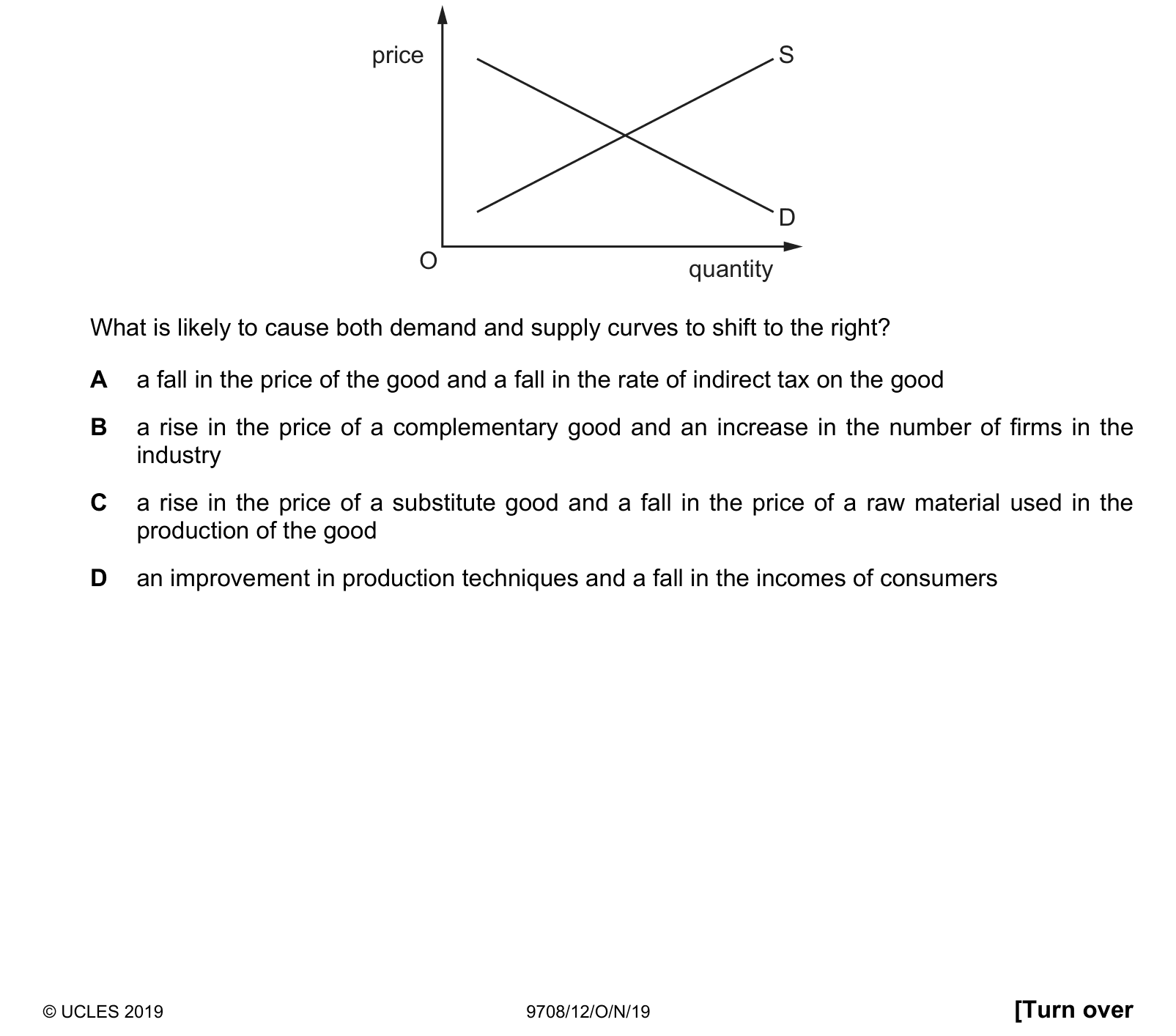
Answer: C.
Cross-board concept practice · originally a CIE 9708 question, used here because the concept is the same. It is not AP Economics past-paper material.
Question 2
The government imposes a specific indirect tax of $1 on each unit of a good sold. How does the imposition of the tax shift the demand or supply curve of the good?
Answer: D.
Cross-board concept practice · originally a CIE 9708 question, used here because the concept is the same. It is not AP Economics past-paper material.
Question 3
The demand for houses in London has caused house prices to rise considerably in the last five years. Many people cannot now afford to buy a house.
What can be concluded from this?
Answer: B.
What the syllabus asks for on this topicWhat this unit covers
What this unit covers
- Demand, supply and market equilibrium.
- Price elasticity of demand and of supply.
- Income elasticity and cross-price elasticity.
- Consumer surplus, producer surplus and total welfare.
- Government intervention: price controls, taxes and subsidies.
This is one of the two heaviest units in AP Microeconomics, and it is also the one whose tools every later unit reuses. Elasticity returns in tax incidence, surplus areas return in every welfare argument, and the shift-versus-movement distinction is tested somewhere in almost every free-response question.
Related AP Economics topics
Not the topic you were looking for? Describe what you are stuck on in your own words and we will take you to the notes that answer it.