Revenues, Costs and Profits
Contents: 11 sections
Revenue
| Measure | Formula | Note |
|---|---|---|
| Total revenue (TR) | Price × quantity | |
| Average revenue (AR) | TR ÷ Q | AR = price, so the AR curve is the demand curve |
| Marginal revenue (MR) | ΔTR ÷ ΔQ | Revenue from one more unit |
Two cases:
A price taker (perfect competition) sells any quantity at the market price, so its demand curve is perfectly elastic and AR = MR = price, both horizontal.
A price maker faces a downward-sloping demand curve. To sell one more unit it must lower the price on every unit, so MR falls faster than AR and lies below it. For a straight-line demand curve, MR has twice the gradient and cuts the horizontal axis halfway along.
The elasticity link:
- Demand elastic → MR positive → cutting price raises TR.
- Demand unit elastic → MR = 0 → TR at a maximum.
- Demand inelastic → MR negative → cutting price reduces TR.
Costs
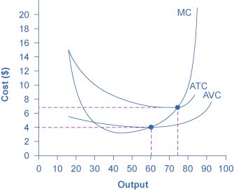
| Cost | Definition |
|---|---|
| Fixed cost | Does not vary with output: rent, insurance, loan interest |
| Variable cost | Varies with output: raw materials, hourly wages |
| Total cost | TC = TFC + TVC |
| Average total cost | ATC = TC ÷ Q, and ATC = AFC + AVC |
| Marginal cost | ΔTC ÷ ΔQ: the cost of one more unit |
Relationships to hold:
- MC cuts AVC and ATC at their minimum points. When MC is below an average, it pulls the average down; when above, it pulls it up.
- AFC falls continuously as fixed cost is spread over more units, so ATC and AVC converge as output rises.
The short run: diminishing returns
- Short run: at least one factor is fixed.
- Long run: all factors are variable.
The law of diminishing returns applies only in the short run: as successive units of a variable factor are added to a fixed factor, the marginal product of the variable factor eventually falls.
- Extra workers are added to a fixed factory
- at first specialisation raises marginal product
- but the fixed capital is spread ever more thinly
- each extra worker adds less than the one before
- marginal product falls
- and since MC is the wage divided by marginal product, marginal cost rises.
That is why the short-run cost curves are U-shaped, and ultimately why the supply curve slopes upwards.
The long run: returns to scale
- Increasing returns to scale: output rises proportionately more than inputs → LRAC falls → economies of scale.
- Constant returns: LRAC flat.
- Decreasing returns: LRAC rises → diseconomies of scale.
The LRAC curve is the envelope of all possible short-run ATC curves, and is also U-shaped, but for an entirely different reason. The short-run U comes from diminishing returns to a fixed factor; the long-run U comes from returns to scale. Confusing the two is the most common error in this topic.
Internal economies of scale (RTFMPM):
| Type | Mechanism |
|---|---|
| Risk-bearing | Diversification across products and markets |
| Technical | Larger, more efficient machinery becomes viable |
| Financial | Big firms borrow more cheaply, being lower-risk |
| Marketing | Advertising and distribution spread over more units |
| Purchasing | Bulk-buying discounts |
| Managerial | Specialist managers, their cost spread over more output |
External economies of scale come from growth of the whole industry: a skilled local labour pool, specialist suppliers clustering, shared infrastructure.
Diseconomies of scale come from control (managers cannot monitor a vast organisation), communication (messages distort through layers) and coordination and motivation (workers feel anonymous).
The minimum efficient scale (MES) is the lowest output at which LRAC is minimised. Where MES is large relative to the market, only a few firms can operate efficiently, which is why some industries are naturally concentrated (3.4).
Profit and the shutdown points
Profit = TR − TC, where economists include opportunity cost in TC.
- Normal profit is the minimum return needed to keep the entrepreneur in the industry. It is a cost of production, so a firm earning exactly normal profit breaks even in economic terms and has no reason to leave.
- Supernormal profit is profit above normal. It attracts entry unless barriers prevent it.
The shutdown conditions, examined directly:
| Condition | Decision |
|---|---|
| AR ≥ ATC | Continue; at least normal profit |
| AVC ≤ AR < ATC | Continue in the short run: the loss is smaller than the fixed costs still payable |
| AR < AVC | Shut down immediately |
The logic: in the short run fixed costs must be paid whether or not the firm produces, so any revenue above variable cost makes a contribution towards them. In the long run all costs are variable, so the firm must cover ATC.
Working the numbers
A price maker faces this demand schedule. Fixed costs are £40.
| Q | Price (= AR) | TR | MR | TC | MC | Profit |
|---|---|---|---|---|---|---|
| 1 | £50 | £50 | £50 | £70 | £30 | −£20 |
| 2 | £45 | £90 | £40 | £95 | £25 | −£5 |
| 3 | £40 | £120 | £30 | £125 | £30 | −£5 |
| 4 | £35 | £140 | £20 | £165 | £40 | −£25 |
Profit is maximised where MR = MC, and here that is between the second and third units, MR falls 40 → 30 while MC rises 25 → 30. Output of 2 or 3 gives the smallest loss of £5.
Three readings the exam wants:
- MR falls twice as fast as AR. Price drops £5 a step; MR drops £10. That is the "twice the gradient" rule as arithmetic, and the reason is that selling one more unit means cutting the price on all the earlier ones too.
- MC is the change in total cost between rows, not TC ÷ Q. Confusing the two is the most common table error.
- The firm is making a loss at every output. It should still produce in the short run provided price covers average variable cost, because fixed costs of £40 are paid either way, closing would lose the full £40, while producing loses only £5.
Revenue maximisation would be a different answer: TR peaks where MR = 0, further right than MR = MC, so output is higher and price lower. That is why a firm pursuing sales or revenue targets rather than profit produces more and charges less, a point consumers benefit from and shareholders do not.
Worked example
A firm faces a market price of £8. Its ATC at current output is £10 and its AVC is £7.
AR (£8) is below ATC (£10), so the firm is making a loss of £2 per unit.
But AR (£8) is above AVC (£7), so each unit contributes £1 towards fixed costs.
Short-run decision: keep producing. Shutting down would mean losing the whole of fixed costs; producing recovers £1 per unit of them, so the loss is smaller by continuing.
Long-run decision: if the price does not recover above £10, all costs become variable and the firm should exit the industry.
Evaluation.
- The judgement depends on whether the low price is temporary or permanent. A cyclical downturn justifies continuing; a permanent shift in demand does not.
- It also depends on the size of sunk costs. Where exit costs are high and unrecoverable, the firm has a stronger reason to continue in the hope of recovery.
- Time period matters for costs too: what is fixed in the short run becomes variable in the long run, so the shutdown threshold itself moves.
- If the firm expects rivals to exit first, remaining could leave it facing a higher price later, a strategic consideration outside the basic model.
Judgement: with AR above AVC the firm should continue in the short run, but the decision is only defensible while the price is expected to recover; otherwise it is delaying an exit that will be more costly later.
Common exam mistakes
- Confusing diminishing returns (short run, one fixed factor) with diseconomies of scale (long run, all variable). This is the biggest discriminator in Theme 3.
- Giving the shutdown point as ATC rather than AVC in the short run.
- Saying normal profit means zero profit. It is zero economic profit and a cost.
- Drawing MC cutting ATC anywhere other than its minimum.
- Saying diminishing returns means total output falls; it is the marginal product that falls.
- Forgetting AR = price = the demand curve.
- Listing economies of scale without explaining how each lowers average cost.
Exam technique
State the time horizon in your first line: short run means a fixed factor and diminishing returns; long run means all variable and returns to scale.
Draw the cost curves accurately, MC through the minimum of AVC and ATC, AFC falling throughout, LRAC U-shaped with MES marked. Most of the marks in this topic attach to a correctly drawn diagram.
For shutdown questions, compare AR against AVC and ATC explicitly and name the time period. For evaluation, use the temporary-versus-permanent distinction and sunk costs.
Quick revision
- AR = price = the demand curve. Price taker: AR = MR = P. Price maker: MR below AR, twice the gradient.
- MR = 0 at maximum TR, where demand is unit elastic.
- ATC = AFC + AVC. MC cuts AVC and ATC at their minimum. AFC falls continuously.
- Short run: one factor fixed → diminishing marginal returns → rising MC → U-shaped SRAC.
- Long run: all variable → returns to scale → U-shaped LRAC.
- Internal economies: Risk-bearing, Technical, Financial, Marketing, Purchasing, Managerial.
- Diseconomies: control, communication, coordination and motivation.
- Normal profit is a cost; supernormal profit attracts entry.
- Short-run shutdown: AR < AVC. Long-run: AR < ATC.
What the syllabus asks for on this topicSpecification points
Specification points
- Total, average and marginal revenue.
- Total, average and marginal cost; short-run and long-run costs.
- The law of diminishing returns and returns to scale; economies and diseconomies of scale.
- Normal and supernormal profit; the shutdown points.
Related Edexcel A-Level topics
Not the topic you were looking for? Describe what you are stuck on in your own words and we will take you to the notes that answer it.