The Labour Market
Contents: 13 sections
The demand for labour

Note which curve the wage line touches, because it is not the one the hiring rule uses. A firm hires up to where the wage equals marginal revenue product, and at Q the marginal revenue product has fallen all the way to zero, so Q is far beyond that point.
What Q marks instead is the limit of viability. At X the wage equals average revenue product, meaning the total wage bill exactly equals the total revenue the workforce generates. Employ one worker more and the firm pays out more than the labour brings in. So the hiring decision is made where W meets MRP, and Q is the point past which employing anyone at all stops making sense.
Labour demand is derived demand, firms want workers not for their own sake but for the output they produce. If demand for the product falls, demand for the labour that makes it falls too.
A profit-maximising firm hires up to the point where the marginal revenue product of labour equals the wage.
MRP = marginal physical product × marginal revenue
MRP measures the extra revenue a firm gains from employing one more worker. It slopes downwards because of the law of diminishing returns (3.1): with capital fixed, each extra worker adds less physical output than the last.
The hiring rule: employ workers up to where MRP = wage. Below that point, the worker adds more revenue than they cost, so hiring raises profit; beyond it, the worker costs more than they contribute.
Determinants of labour demand: demand for the final product, labour productivity, the price of capital (labour and capital may be substitutes or complements), and the wage itself.
Elasticity of labour demand is higher when: the product's PED is high; labour is a large proportion of total costs; capital substitutes easily for labour; and the time period is long.
The supply of labour
Supply to an occupation slopes upwards: a higher wage attracts workers from other jobs and induces existing workers to work longer.
Determinants: the wage; wages in alternative occupations; non-monetary characteristics (danger, hours, status, satisfaction); the qualifications and training required; barriers to entry such as professional licensing; the size and mobility of the population; and social attitudes.
Elasticity of labour supply is low where training is long and qualifications are demanding, which is why surgeons' supply cannot expand quickly, and why their wages are high.
Mobility of labour matters throughout:
- Occupational immobility: workers lack the skills to move between jobs, the main cause of structural unemployment (6.2).
- Geographical immobility: housing costs, family ties and information gaps stop workers moving between regions.
Wage determination in a competitive labour market
With many small employers and many workers, no single participant can influence the wage.
- The market wage is set where labour demand meets labour supply
- each individual firm is a wage taker, facing a perfectly elastic supply of labour at that wage
- so wage = ACL = MCL
- and the firm employs where MRP = wage.
This produces the allocatively efficient level of employment: workers are paid exactly the value of what they contribute at the margin.
Monopsony
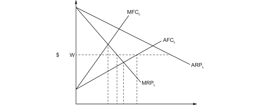
Work the diagram in that order. The monopsonist hires where MFC equals MRP, the leftmost dashed line, because that is where the cost of the next worker stops being covered by what that worker adds. It then pays the wage that this many workers are willing to accept, which is read off the AFC curve directly below that point, not off MFC. A competitive market would instead settle where AFC meets MRP, further right, so monopsony delivers both lower employment and a lower wage.
The wage line W is drawn higher than either, which is what makes this a question rather than an illustration: it is a wage imposed on the market, and the exercise is to work out what happens to employment when the employer can no longer choose the wage.
A monopsony is a single (or dominant) buyer of labour, a large public employer, or the only significant employer in a town.
Because it is large relative to the market, it faces the upward-sloping market supply curve of labour. To attract one more worker it must raise the wage, and, if it cannot discriminate, raise it for everyone already employed.
Therefore the marginal cost of labour (MCL) lies above the average cost of labour (ACL), just as MR lies below AR for a monopolist.
- The monopsonist hires where MRP = MCL, then reads the wage down to the supply (ACL) curve
- the result is lower employment and a lower wage than in a competitive market
- workers are paid less than their MRP, which is exploitation in the technical sense, and there is a welfare loss.
Trade unions
A trade union is an organised association of workers bargaining collectively.
In a competitive labour market, a union raising the wage above equilibrium creates excess supply of labour, the classic trade-off of higher wages for those employed, at the cost of fewer jobs. The employment loss is larger where labour demand is elastic.
In a monopsonistic labour market the result reverses, and this is the highest-value analysis in the topic:
- A union facing a monopsonist creates a bilateral monopoly
- it can raise the wage towards the competitive level
- because the employer can no longer depress the wage by restricting hiring, the effective marginal cost of labour becomes flat at the negotiated wage
- so both the wage AND employment can rise at the same time.
A union's power depends on: its membership density, the elasticity of labour demand (the more inelastic, the more it can extract), the firm's profitability, the legal framework, and the state of the macroeconomy.
Unions may also raise productivity, by giving workers voice, reducing turnover, and negotiating training, which shifts MRP right and can raise wages without costing jobs.
The national minimum wage
A minimum wage is a legal price floor, set above the equilibrium wage.
The standard analysis: it creates excess supply, more workers want jobs at that wage than firms wish to hire, so it causes unemployment, concentrated among the low-skilled and the young. The effect is larger where labour demand is elastic.
The counter-arguments:
- If the employer is a monopsonist, a minimum wage set between the monopsony wage and the competitive wage raises both wages and employment.
- Higher pay may raise motivation and productivity (efficiency wage theory), shifting MRP right and offsetting the cost.
- Lower turnover cuts recruitment and training costs.
- Higher incomes for low earners raise consumption, and with a high marginal propensity to consume this raises aggregate demand and hence derived demand for labour (7.1).
- It reduces in-work poverty and cuts the cost of in-work benefits to the taxpayer.
Judgement turns on the level at which it is set and how much monopsony power employers actually have.
Wage differentials
Wages differ between occupations, regions, genders and ethnic groups because of:
- Different MRP: driven by skills, education and the value of the output.
- Different elasticity of supply: long training and licensing restrict supply and raise pay.
- Compensating differentials: dangerous, unpleasant or unsociable work pays more, other things equal.
- Immobility of labour, both occupational and geographical, preventing wages from equalising.
- Trade union power in some occupations but not others.
- Discrimination, which lowers the demand for, or pay of, particular groups regardless of MRP.
- Imperfect information about available jobs and pay.
Working the numbers
Marginal revenue product is what the firm is buying when it hires.
MRP = marginal physical product × marginal revenue (= price, selling competitively)
Output sells at £10:
| Workers | Total output | MPP | MRP |
|---|---|---|---|
| 1 | 9 | 9 | £90 |
| 2 | 20 | 11 | £110 |
| 3 | 29 | 9 | £90 |
| 4 | 35 | 6 | £60 |
| 5 | 38 | 3 | £30 |
At a market wage of £80, the firm employs 3, the third worker adds £90, the fourth only £60. Raise the wage to £100 and it employs 2.
MPP rises then falls, so MRP does too: that is diminishing returns, and it is why labour demand slopes downward.
Monopsony
A sole employer faces the upward-sloping market labour supply, so hiring one more means raising the wage for everyone already employed. Marginal cost of labour therefore exceeds the wage:
| Workers | Wage | Total labour cost | MCL |
|---|---|---|---|
| 1 | £50 | £50 | £50 |
| 2 | £60 | £120 | £70 |
| 3 | £70 | £210 | £90 |
| 4 | £80 | £320 | £110 |
Hiring the third worker costs £90: £70 for them, plus the £10 rise given to each of the two already there.
Against the MRP schedule above, the monopsonist hires while MRP ≥ MCL:
Worker 3: MRP £90 ≥ MCL £90 → hire. Worker 4: £60 < £110 → stop.
3 workers at a wage of £70, read the wage down to the supply curve. Never off MCL.
A competitive labour market with the same supply schedule would pay £80 and employ 3. So monopsony delivers the lower wage, which is the exam's point, and it is why a minimum wage set at £80 here would raise pay without costing jobs, exactly reversing the usual conclusion.
Worked example
A government raises the national minimum wage significantly in a region where one large employer dominates local hiring.
The competitive prediction:
- The wage floor sits above the competitive equilibrium
- quantity of labour demanded falls, quantity supplied rises
- excess supply, i.e. unemployment
- the low-skilled are hit hardest, since their MRP is closest to the new wage.
The monopsony prediction:
- The dominant employer was hiring where MRP = MCL and paying a wage below MRP
- the minimum wage removes its ability to depress pay by restricting hiring
- the effective MCL becomes horizontal at the legal wage
- the firm now hires where MRP = the minimum wage
- both the wage and employment rise, and the exploitation gap closes.
Evaluation.
- Which prediction holds depends on the degree of monopsony power and on where the minimum wage is set. Between the monopsony and competitive wage, employment rises; above the competitive wage, it falls.
- The elasticity of labour demand governs the size of any job losses, inelastic demand means the employment cost is small.
- Firms may respond by substituting capital for labour, cutting hours rather than headcount, or raising prices, so measured unemployment understates the adjustment.
- Empirical evidence on real minimum wages has generally found smaller employment effects than the simple competitive model predicts, which is itself evidence that monopsony power is widespread.
Judgement: a moderate minimum wage in a monopsonistic labour market raises pay and employment together; an aggressive one in a competitive labour market with elastic demand costs jobs. The policy is not right or wrong in principle, it depends on the level and the market structure.
Common exam mistakes
- Forgetting that labour demand is derived.
- Confusing MRP with marginal physical product, MRP is measured in revenue.
- Drawing MCL below ACL for a monopsonist; it must be above.
- Reading the monopsonist's wage off the MRP curve instead of down to the supply curve.
- Claiming a minimum wage always causes unemployment, ignoring monopsony and efficiency wages.
- Saying unions always cost jobs, under monopsony they can raise wages and employment.
- Explaining wage differentials only by MRP, ignoring elasticity of supply and immobility.
Exam technique
State whether the labour market is competitive or monopsonistic before drawing anything, the entire analysis and conclusion depend on it.
For monopsony, label MRP, ACL and MCL carefully, mark the intersection of MRP and MCL, and drop down to ACL for the wage. Shade the gap between MRP and the wage as the exploitation.
For any minimum wage or union question, give both the competitive and monopsony cases and then judge between them using elasticity, the level of the wage, and the evidence. That two-model structure is what top answers do.
Quick revision
- Labour demand is derived; firms hire where MRP = wage.
- MRP = marginal physical product × marginal revenue; it falls due to diminishing returns.
- Labour demand is more elastic when product PED is high, labour is a big share of costs, and capital substitutes easily.
- Competitive market: wage = ACL = MCL; workers paid their MRP.
- Monopsony: single buyer, MCL above ACL, hires where MRP = MCL, pays down on the supply curve → lower wage and employment, workers paid below MRP.
- Unions in a competitive market: higher wage, fewer jobs. Against a monopsonist: higher wage and more jobs.
- Minimum wage: causes unemployment in a competitive market; can raise wages and employment under monopsony.
- Wage differentials: MRP, elasticity of supply, compensating differentials, immobility, union power, discrimination.
Check you have it
Question 1
Figure 8 shows the market demand (D L ) and supply (S L ) of labour in a labour market with a trade union. The initial trade union negotiated wage is W 2 . Figure 8 The trade union negotiates an increase in the wage from W 2 to W 3 . All other things being equal, unemployment in this labour market will increase by
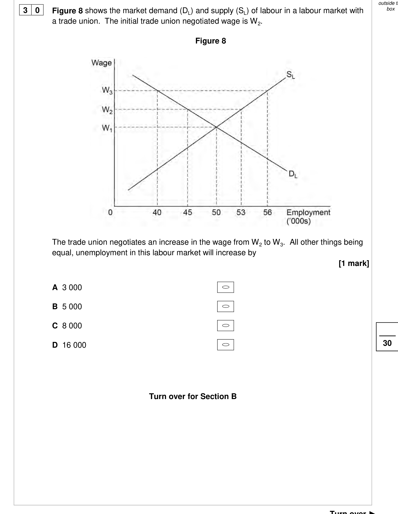
Answer: C.
Question 2
The UK’s labour productivity increases by only 10% over a five year period. Over the same period its main trading partners increase their productivity by 25%. All other things being equal, the most likely consequence for the UK is
Answer: C.
Question 3
Increased output results from specialisation and the division of labour because they enable
Answer: B.
What the syllabus asks for on this topicSpecification points
Specification points
- The demand for and supply of labour; marginal revenue product.
- Wage determination in competitive and non-competitive markets.
- Monopsony, trade unions, the minimum wage and wage differentials.

Related AQA A-Level topics
Not the topic you were looking for? Describe what you are stuck on in your own words and we will take you to the notes that answer it.