Production and Costs
Contents: 8 sections
Production and productivity
- Production is the total output produced.
- Productivity is output per unit of input, usually output per worker or per hour.
The distinction matters: a firm can raise production simply by hiring more workers without raising productivity at all. Only higher productivity lowers unit costs and improves competitiveness, which is why it dominates supply-side policy (9.3).
Determinants of labour productivity: education and training, the quantity and quality of capital each worker has, technology, management, and worker motivation.
Specialisation and the division of labour raise productivity because workers concentrate on the task they perform best, become quicker through repetition, need training in only one operation, and lose no time switching between tasks. Against this, specialisation can cause boredom and demotivation, makes workers occupationally immobile if the industry declines, and creates interdependence, one broken link halts the whole process.
The short run and the law of diminishing returns
- Short run: at least one factor is fixed, so output can only be raised by adding variable factors.
- Long run: all factors are variable, and the scale of the whole operation can change.
The law of diminishing returns applies only in the short run: as successive units of a variable factor are added to a fixed factor, the marginal product of the variable factor eventually falls.
- Extra workers are added to a fixed factory
- at first specialisation raises marginal product
- but the fixed capital is eventually spread too thinly
- each extra worker adds less than the one before
- marginal product falls.
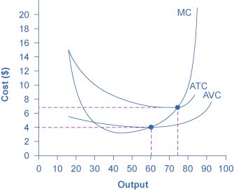
Because marginal cost is the wage divided by marginal product, falling marginal product means rising marginal cost. This is the reason the short-run cost curves are U-shaped, and ultimately the reason the supply curve slopes upwards (2.1).
The relationships to hold:
- MC cuts AVC and ATC at their minimum points. When marginal cost is below average cost, the average is pulled down; when above; it is pulled up.
- AFC falls continuously as output rises, because fixed cost is spread over more units.
- ATC = AFC + AVC, so ATC and AVC converge as output rises.
| Cost | Definition |
|---|---|
| Fixed cost | Does not vary with output: rent, insurance, loan interest |
| Variable cost | Varies with output: raw materials, wages of hourly staff |
| Total cost | TC = TFC + TVC |
| Average total cost | ATC = TC ÷ Q |
| Marginal cost | The cost of producing one more unit: ΔTC ÷ ΔQ |
Building the cost table
AQA sets these as data questions, and the whole table follows from fixed costs plus a variable-cost column. With fixed costs of £60:
| Q | TVC | TC | MC | AVC | ATC |
|---|---|---|---|---|---|
| 0 | £0 | £60 | : | : | : |
| 1 | £40 | £100 | £40 | £40.00 | £100.00 |
| 2 | £70 | £130 | £30 | £35.00 | £65.00 |
| 3 | £110 | £170 | £40 | £36.67 | £56.67 |
| 4 | £170 | £230 | £60 | £42.50 | £57.50 |
Four things to read off it, each of which the exam asks:
- MC is the change in total cost between rows, not a total divided by anything. That single error accounts for most lost marks on cost tables.
- MC falls then rises: increasing returns to the variable factor at first, then diminishing returns from the third unit onwards. The cost curve's U-shape is the law of diminishing returns in numbers.
- AVC bottoms out at Q = 2 (£35) and ATC at Q = 3 (£56.67): AVC turns first, because falling average fixed cost is still dragging ATC down after AVC has begun to rise.
- The gap between ATC and AVC is average fixed cost: at Q = 3, £56.67 − £36.67 = £20, which is £60 ÷ 3. It shrinks towards zero as output rises, "spreading the overhead", and never reaches it.
The long run: returns to scale
In the long run every factor can be varied, so the firm chooses its scale.
- Increasing returns to scale: output rises proportionately more than inputs → long-run average cost falls → economies of scale.
- Constant returns: output rises in proportion → LRAC is flat.
- Decreasing returns: output rises proportionately less → LRAC rises → diseconomies of scale.
The LRAC curve is the envelope of all possible short-run ATC curves, and is likewise U-shaped, but for an entirely different reason from the short-run curve. The short-run U comes from diminishing returns to a fixed factor; the long-run U comes from returns to scale. Confusing the two is the most common error in this topic.
Internal economies of scale (mnemonic: RTFMPM)
| Type | Mechanism |
|---|---|
| Risk-bearing | A large firm diversifies across products and markets |
| Technical | Larger, more efficient machinery and production lines become viable |
| Financial | Big firms borrow at lower interest rates, as they are lower-risk |
| Marketing | Advertising and distribution costs are spread over more units |
| Purchasing | Bulk-buying discounts on inputs |
| Managerial | Specialist managers can be employed and their cost spread |
External economies of scale arise from the growth of the whole industry, not the firm, a skilled local labour pool, specialist suppliers clustering nearby, and shared infrastructure.
Diseconomies of scale come from control (managers cannot monitor a vast organisation), communication (messages distort across layers of hierarchy), and coordination and motivation (workers feel anonymous and alienated in a huge firm).
The minimum efficient scale (MES) is the lowest output at which LRAC is minimised. Where MES is large relative to the market, only a few firms can operate efficiently, which is why some industries are naturally concentrated (4.1).
Worked example
A car manufacturer doubles the size of its plant and its workforce, and output more than doubles.
- All factors have been varied, so this is the long run
- output rises proportionately more than inputs
- increasing returns to scale
- LRAC falls.
The sources, which the question wants named:
- Technical: a robotic assembly line only makes sense at high volume; its cost is now spread over far more cars.
- Purchasing: steel and components are bought in larger contracts at lower unit prices.
- Financial: the larger firm borrows more cheaply to fund the expansion.
- Marketing: the advertising budget is spread across a much larger output.
- Lower average cost
- the firm can cut price and still make normal profit
- it gains market share, raising output further and reinforcing the cost advantage.
Evaluation.
- The gain has limits. Beyond the minimum efficient scale, diseconomies appear: coordinating two plants and a doubled workforce strains management, and communication between layers degrades.
- The cost advantage is only realised if the extra output can actually be sold. If demand does not grow with capacity, the plant runs below capacity and average fixed costs per unit rise instead of falling.
- Economies of scale can become a barrier to entry, entrenching the firm's market power to the detriment of consumers, a link to 4.1 worth making.
- In the short run, before the new plant is complete, adding workers to the existing factory would run into diminishing returns and rising marginal cost. The two effects operate over different time horizons.
Judgement: the expansion lowers unit costs while the firm is below MES and demand supports the volume; beyond that, diseconomies and unsold capacity reverse the advantage.
Common exam mistakes
- Confusing diminishing returns (short run, one fixed factor) with diseconomies of scale (long run, all factors variable). This is the single biggest discriminator.
- Confusing production (total output) with productivity (output per input).
- Saying diminishing returns means total output falls; it is the marginal product that falls; total output usually still rises.
- Drawing MC cutting ATC anywhere other than its minimum.
- Treating external economies as internal, external ones come from the industry, not the firm.
- Listing economies of scale without explaining how each lowers average cost.
Exam technique
State the time horizon in your first line. Short run means at least one fixed factor and diminishing returns; long run means all variable and returns to scale.
Draw the cost curves accurately: MC through the minimum of AVC and ATC, AFC falling throughout, and a U-shaped LRAC with MES marked.
For evaluation, use the limits of scale (diseconomies beyond MES), demand (cost savings need volume), and the link to market structure (economies of scale as a barrier to entry).
Quick revision
- Production = total output. Productivity = output per input.
- Division of labour raises productivity but causes boredom, immobility and interdependence.
- Short run: one factor fixed → diminishing marginal returns → rising MC → U-shaped SRAC.
- MC cuts AVC and ATC at their minimum. AFC falls continuously.
- Long run: all factors variable → returns to scale → U-shaped LRAC.
- Internal economies: Risk-bearing, Technical, Financial, Marketing, Purchasing, Managerial.
- External economies come from industry growth: skilled labour pool, suppliers, infrastructure.
- Diseconomies: control, communication, coordination and motivation.
- MES = lowest output at minimum LRAC; a large MES concentrates the industry.
Check you have it
Question 1
Table 2 shows the relationship between the number of workers employed by a firm and the total output of a product. The amount of other factors of production employed remains the same. Number of workers / Total output: 1/8, 2/28, 3/54, 4/82, 5/103, 6/103, 7/99. For this firm, diminishing marginal returns to labour occur when the
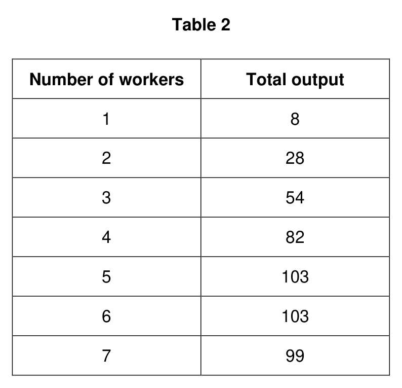
Answer: B.
What the syllabus asks for on this topicSpecification points
Specification points
- Production and productivity; specialisation and the division of labour.
- The law of diminishing returns (short run).
- Returns to scale and economies/diseconomies of scale (long run).
Related AQA A-Level topics
Not the topic you were looking for? Describe what you are stuck on in your own words and we will take you to the notes that answer it.