Aggregate Supply
Contents: 9 sections
Short-run aggregate supply
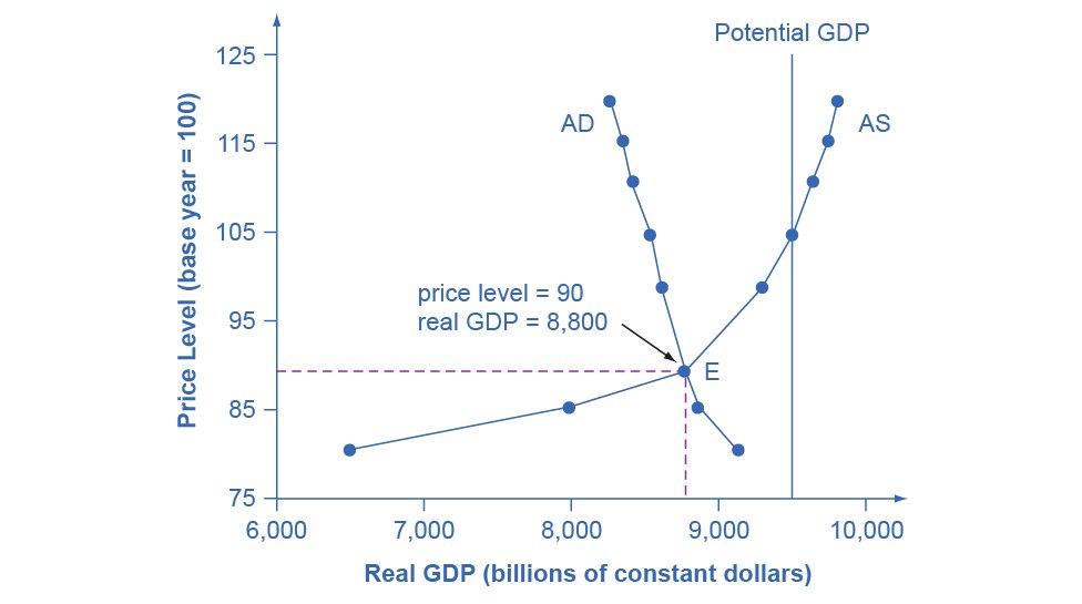
SRAS shows total planned output at each price level when factor prices, especially wages, are fixed.
It slopes upwards: with input costs fixed, a higher price level raises profit margins, so firms expand output.
Shifters of SRAS are anything that changes firms' costs of production:
| Factor | Effect |
|---|---|
| Wage rates | Higher wages → SRAS left |
| Raw material and energy prices | Higher → SRAS left |
| Exchange rate | Depreciation raises imported input costs → SRAS left |
| Indirect taxes and regulation | Higher → SRAS left |
| Subsidies to producers | SRAS right |
| Productivity | Higher output per worker lowers unit costs → SRAS right |
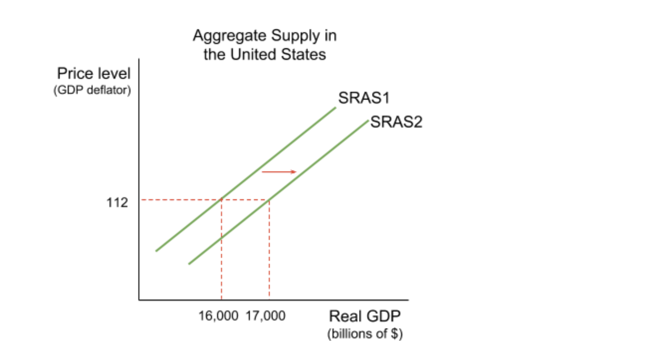
A leftward SRAS shift is a supply shock, and it raises the price level while lowering output, cost-push inflation (6.2), and if severe, stagflation.
Long-run aggregate supply
LRAS shows the economy's productive potential, what it can produce when all resources are fully and efficiently employed. It is independent of the price level, and corresponds to the PPF (1.1).
Shifters of LRAS are anything that changes the quantity or quality of the factors of production:
- Investment in capital stock and infrastructure.
- Technological progress.
- Education, training and skills: human capital.
- The size of the labour force: demographics, participation rates, net migration.
- Enterprise and incentives, including tax structure.
- Discovery of natural resources.
- Institutions: property rights, competition, the rule of law.
- Labour market flexibility and reduced factor immobility.
These are exactly the targets of supply-side policy (9.3).
Classical and Keynesian views
This disagreement is the most examinable idea in the topic, because the two models give opposite policy conclusions.
The classical (monetarist) LRAS is vertical at the full-employment level of output.
The reasoning: markets clear. Any deviation from full employment is temporary, because wages and prices are flexible and adjust to restore equilibrium. Output is therefore determined solely by supply-side factors.
- An increase in AD raises output only in the short run. Higher prices erode real wages
- workers demand higher nominal wages
- SRAS shifts left
- output returns to the full-employment level at a higher price level. Demand management is therefore purely inflationary in the long run, and only supply-side policy raises output.
The Keynesian LRAS has three sections:
- A horizontal (perfectly elastic) section at low output, with mass unemployment and substantial spare capacity, firms can raise output without any rise in the price level.
- An upward-sloping section, as capacity is approached, bottlenecks and shortages appear, so expansion raises both output and prices.
- A vertical section at full capacity, no further output is possible, so extra demand is entirely inflationary.
The reasoning: wages are sticky downwards, because of contracts, minimum wages, union resistance and reluctance to cut nominal pay. An economy can therefore become stuck in a deflationary gap, an equilibrium below full employment that does not self-correct.
On the horizontal section, an increase in AD raises real output with no inflation. Demand management is therefore both effective and necessary, since the market will not correct itself.
The policy implication, which is the point of learning both:
| Classical | Keynesian | |
|---|---|---|
| Long-run output determined by | Supply-side factors only | AD as well, when below capacity |
| Demand management | Inflationary, ineffective | Effective when there is spare capacity |
| Recommended policy | Supply-side: tax cuts, deregulation, flexibility | Demand-side first, to close the output gap |
| Self-correcting? | Yes, via flexible wages and prices | No: wages are sticky downwards |
The reconciliation: which view is right depends on where the economy is operating. In a deep recession with a large negative output gap the Keynesian analysis fits; near full capacity the classical one does. Saying this explicitly is the highest-level move available in an essay on this topic.
Macroeconomic equilibrium
Equilibrium is where AD = AS, determining the equilibrium price level and real output.
- Short-run equilibrium: AD = SRAS. Output can be above or below the full-employment level.
- Long-run equilibrium: AD = SRAS = LRAS, with output at potential.
Reflation is a rightward AD shift; deflationary pressure a leftward one. The split of any AD shift between output and prices depends entirely on which part of AS the economy is on, which is why identifying the output gap is the first step in any macro answer.
Worked example
A government cuts income tax to stimulate a sluggish economy.
The Keynesian analysis, assuming a large negative output gap:
- Lower income tax raises disposable income
- consumption rises
- AD shifts right, amplified by the multiplier (7.1)
- because the economy is on the horizontal section of LRAS with substantial spare capacity
- real output and employment rise with almost no increase in the price level
- the negative output gap closes.
The classical analysis:
- The economy is already at full employment on a vertical LRAS
- AD shifts right
- in the short run output rises above potential and unemployment falls below its natural rate
- but the higher price level erodes real wages
- workers bargain for higher nominal wages
- SRAS shifts left
- output returns to the full-employment level
- the only lasting effect is a higher price level.
Evaluation.
- Everything depends on the size of the output gap, and potential output is estimated, not observed, so the same policy can be either effective or purely inflationary depending on a number nobody knows precisely.
- The tax cut may also have supply-side effects: better incentives to work and to enter the labour force could shift LRAS right, in which case even the classical model permits a lasting output gain.
- It must be financed. Higher borrowing raises the deficit, and may cause crowding out, although that objection is weak when interest rates are at their floor and private demand is depressed.
- The distributional effect matters for the size of the stimulus: cuts targeted at low earners, who have a higher MPC, deliver more demand per pound forgone.
- Time lags mean the stimulus may arrive after recovery has begun, when the classical prediction becomes the relevant one.
Judgement: with a genuine and large negative output gap, the tax cut raises real output at little inflationary cost; near capacity it is inflationary and the supply-side effects are the only durable gain. The right policy therefore depends on the diagnosis, not on the model chosen in advance.
Common exam mistakes
- Drawing LRAS as upward-sloping; it is vertical (classical) or three-sectioned (Keynesian).
- Shifting LRAS for a change in production costs. Costs shift SRAS; only capacity shifts LRAS.
- Presenting the Keynesian LRAS with only the horizontal section, omitting the upward-sloping and vertical parts.
- Saying the classical model means demand policy never works, it works in the short run.
- Ignoring where on the AS curve the economy currently sits, which determines the entire outcome.
- Confusing a movement along AS (price level change) with a shift.
Exam technique
Draw AD, SRAS and LRAS on the same diagram and mark the full-employment level of output. Almost every macro question in this section is answered by identifying where the current equilibrium sits relative to it.
State which model you are using and why, "given the large negative output gap described in the extract, the Keynesian analysis is the relevant one."
For evaluation, contrast the two models directly, and conclude that the answer depends on the output gap, the time horizon, and whether the policy also has supply-side effects.
Quick revision
- SRAS slopes up; shifted by costs: wages, raw materials, exchange rate, taxes, productivity.
- LRAS shows productive potential; shifted by the quantity and quality of factors: investment, technology, skills, labour force, institutions.
- Classical LRAS is vertical: output is supply-determined; demand management is inflationary in the long run.
- Keynesian LRAS has three sections: horizontal, upward-sloping, vertical, because wages are sticky downwards.
- On the horizontal section, AD stimulus raises output with no inflation.
- Equilibrium where AD = AS; the split between output and prices depends on where on AS the economy is.
- The models are reconciled by the size of the output gap.
What the syllabus asks for on this topicSpecification points
Specification points
- Short-run and long-run aggregate supply (SRAS, LRAS).
- The factors that shift SRAS and LRAS.
- Keynesian and classical views of LRAS; macroeconomic equilibrium.
Related AQA A-Level topics
Not the topic you were looking for? Describe what you are stuck on in your own words and we will take you to the notes that answer it.