Demand, Supply and Elasticities
Contents: 12 sections
Demand
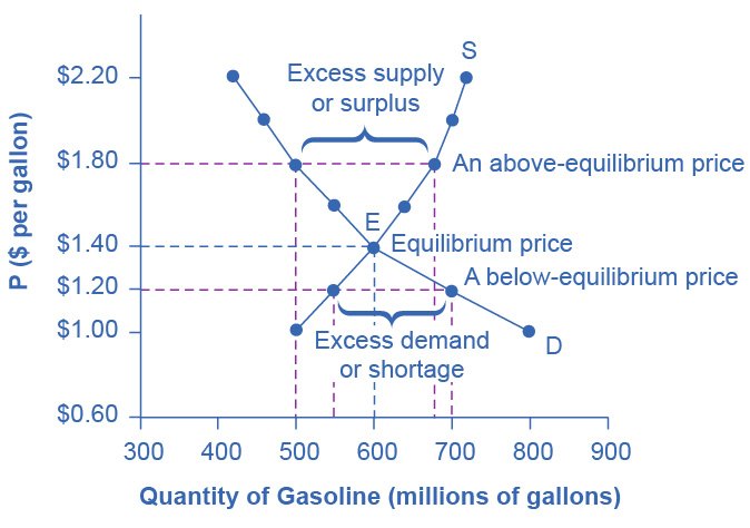
Demand is the quantity consumers are willing and able to buy at each price in a given period. The demand curve slopes downwards because of:
- Diminishing marginal utility: each extra unit yields less satisfaction, so consumers pay less for it (1.2).
- The income effect: a lower price raises real income, so more can be bought.
- The substitution effect: a lower price makes the good cheaper relative to substitutes.
The distinction AQA tests constantly:
- A change in the good's own price causes a movement along the curve, an extension or contraction of demand.
- A change in anything else shifts the curve, an increase or decrease in demand.
Shifters of demand (PIRATES): Population, Income, Related goods (substitutes and complements), Advertising and tastes, Taxes and subsidies on consumers, Expectations of future prices, Seasons.
A demand curve is also a marginal benefit curve: its height at any quantity is what the marginal consumer is willing to pay, which is what that unit is worth to them. That reading is what makes consumer surplus and the welfare analysis in 2.3 and 5.1 possible.
Supply
Supply is the quantity producers are willing and able to sell at each price. It slopes upwards because higher prices raise profitability and cover the rising marginal costs of expanding output (3.1).
Shifters of supply: costs of production, technology, productivity, indirect taxes and subsidies, the number of firms in the market, weather and shocks, and the prices of goods in joint or competing supply.
Correspondingly, the supply curve is the marginal cost curve, which is why price equalling marginal cost at equilibrium is the definition of allocative efficiency.
Price elasticity of demand (PED)
PED = %Δ quantity demanded ÷ %Δ price
PED is always negative for a normal downward-sloping demand curve; quote the sign or refer to the modulus.
| Value | Name | Meaning |
|---|---|---|
| 0 | Perfectly inelastic | Quantity does not respond at all |
| Between 0 and −1 | Inelastic | Quantity changes proportionately less than price |
| −1 | Unit elastic | Proportional change is equal |
| Beyond −1 | Elastic | Quantity changes proportionately more than price |
| ∞ | Perfectly elastic | Any price rise loses all sales |
Determinants (SPLAT): Substitutes available, Proportion of income spent, Luxury or necessity, Addictiveness and habit, Time period. Demand is more elastic in the long run, because consumers find substitutes.
The link to revenue is the highest-value application:
| Price rises | Price falls | |
|---|---|---|
| Inelastic demand | Revenue rises | Revenue falls |
| Elastic demand | Revenue falls | Revenue rises |
Worked calculation
A firm raises price from £10 to £12 and quantity demanded falls from 500 to 450.
%ΔP = (12 − 10) ÷ 10 × 100 = +20%
%ΔQd = (450 − 500) ÷ 500 × 100 = −10%
PED = −10 ÷ 20 = −0.5 → |PED| < 1, so demand is inelastic
Check against revenue, which is the interpretation the marks are for:
Before: £10 × 500 = £5,000. After: £12 × 450 = £5,400.
Revenue rose by £400, or 8%, exactly as inelastic demand predicts. Quantify it directly by multiplying the factors, 1.20 × 0.90 = 1.08, rather than adding the percentages: adding gives the right direction and the wrong number.
PED is not constant along a demand curve
On a straight-line demand curve the slope is fixed but PED is not, because it is a ratio of percentage changes and the base values shift as you move along it:
- Upper section (high price, low quantity), elastic.
- Midpoint: unit elastic, and where total revenue is at its maximum.
- Lower section (low price, high quantity), inelastic.
So "demand for this good is elastic" is never a complete statement without saying where on the curve. It also explains why a firm on the inelastic portion should always raise price: it gains revenue and cuts costs at the same time.
Income elasticity of demand (YED)
YED = %Δ quantity demanded ÷ %Δ income
| YED | Type of good |
|---|---|
| Positive | Normal good: demand rises with income |
| Positive and greater than 1 | Luxury (income-elastic): demand rises faster than income |
| Positive but less than 1 | Necessity (income-inelastic) |
| Negative | Inferior good: demand falls as income rises |
Worked calculation. Real incomes rise 5% and demand for restaurant meals rises 12%.
YED = 12 ÷ 5 = +2.4 → positive and greater than 1, so a normal luxury good.
The planning implication is the point of the question: a 2.4 reading means a 5% fall in incomes during a recession would cut demand by around 12%. Restaurants are therefore highly cycle-exposed, and should build cash reserves in upswings.
YED matters for firms planning for the economic cycle: luxury producers boom in an upswing and suffer badly in a recession, while producers of necessities and inferior goods are far more stable. Firms with a diversified portfolio across YED values smooth their revenue.
Cross elasticity of demand (XED)
XED = %Δ quantity demanded of A ÷ %Δ price of B
| XED | Relationship |
|---|---|
| Positive | Substitutes: B dearer, so more A demanded |
| Negative | Complements: B dearer, so less A demanded |
| Zero | Unrelated goods |
Worked calculation. The price of tea rises 10% and demand for coffee rises 4%.
XED = 4 ÷ 10 = +0.4 → positive, so substitutes, but weakly so.
The larger the modulus, the closer the relationship. A firm with a high positive XED against a rival is highly vulnerable to that rival's pricing; a low figure like 0.4 says the two are only loose alternatives, so a rival's price cut is a limited threat.
Price elasticity of supply (PES)
PES = %Δ quantity supplied ÷ %Δ price
PES is positive for an upward-sloping supply curve.
Worked calculation. Price rises from £20 to £24 and quantity supplied rises from 1,000 to 1,100.
%ΔP = +20%, %ΔQs = +10%
PES = 10 ÷ 20 = 0.5 → inelastic supply
Determinants:
- Time period: the single most important. Supply is far more elastic in the long run, when firms can build capacity.
- Spare capacity: idle machines and workers make supply elastic.
- Stocks: goods that can be stored have elastic supply; fresh produce does not.
- Factor mobility: how easily resources can be switched into this good.
- Production lags: agriculture and mining have very inelastic short-run supply.
Reading PES off a straight-line supply curve is quicker than calculating, and AQA has asked it:
| Where the curve cuts | PES |
|---|---|
| Through the origin | Exactly 1 at every point |
| The price axis | Greater than 1: elastic |
| The quantity axis | Less than 1: inelastic |
Note this is unlike demand, where elasticity varies along a single straight line. Steepness alone tells you nothing about PES.
Elasticity and tax incidence
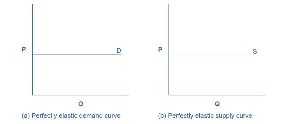
Who actually bears an indirect tax is settled by relative elasticity, not by who hands the money to the government:
The more inelastic side of the market bears the greater share, because it has fewer alternatives and cannot escape by changing behaviour.
Push it to the limits and it is obvious. With perfectly inelastic demand, consumers pay the whole tax. With perfectly elastic demand, producers absorb all of it, since any attempt to pass it on loses every customer.
Elasticity also decides the size of the welfare loss: the more elastic either side, the further quantity falls, and the bigger the triangle. A tax on a good with very inelastic demand raises a lot of revenue and distorts behaviour very little, which is exactly why such goods are taxed, and exactly why those taxes change behaviour so weakly.
Worked example
A government imposes a specific indirect tax on cigarettes to raise revenue and cut consumption.
- The tax raises firms' costs
- supply shifts left
- the equilibrium price rises and quantity falls.
Why the outcome depends on PED:
- Demand for cigarettes is highly inelastic, few substitutes, addictive, a small proportion of income for most smokers.
- So the quantity falls proportionately less than the price rises → consumption barely falls, but tax revenue rises substantially.
- Because demand is inelastic relative to supply, most of the tax incidence falls on consumers, who absorb it through a higher price.
Evaluation.
- The policy succeeds as a revenue measure and largely fails as a consumption measure, an inherent tension, since a tax that genuinely stopped people smoking would raise little revenue.
- The tax is regressive: it takes a larger share of income from poorer smokers.
- It may create a black market, so measured consumption falls further than actual consumption.
- In the long run PED rises, as substitutes such as vaping emerge and habits change, so consumption falls more over time than the short-run figures suggest.
Judgement: with inelastic demand, taxation is an efficient revenue instrument but a weak behavioural one in the short run. Pairing it with information provision and substitutes, which raise PED, makes the consumption objective attainable.
Common exam mistakes
- Confusing a movement along the curve with a shift. Only the good's own price causes a movement.
- Dropping the sign in elasticity answers, the sign carries the meaning in YED and XED.
- Saying an elasticity is "high" without saying elastic or inelastic relative to 1.
- Treating "inferior good" as low quality; it means demand falls as income rises.
- Adding percentage changes to find the revenue effect instead of multiplying the factors.
- Treating a whole demand curve as having one elasticity.
- Judging PES from the steepness of a straight-line supply curve rather than which axis it cuts.
- Assuming whoever pays the tax to the government bears it.
- Forgetting the time period, the strongest determinant of both PED and PES.
- Calculating elasticity from absolute changes rather than percentage changes.
Exam technique
Show the formula, substitute, and interpret, the interpretation carries the analysis marks, not the arithmetic.
Where revenue is involved, compute it both ways: state the elasticity conclusion, then verify with the actual before-and-after figures. Agreement between the two is the strongest possible evidence you have understood the relationship rather than recalled the table.
Use a supply and demand diagram for any shift question, labelling the original and new equilibrium prices and quantities.
For evaluation, the reliable angles are time period (elasticities rise in the long run), the reliability of the elasticity estimate (it is based on past data and may not hold after a large price change), and the range over which it applies (PED varies along a straight-line demand curve).
Quick revision
- Own price → movement along. Anything else → shift.
- Demand is a marginal benefit curve; supply is a marginal cost curve.
- PED = %ΔQd ÷ %ΔP, negative. Determinants: SPLAT.
- Inelastic demand: raise price to raise revenue. Elastic: cut price to raise revenue.
- Quantify revenue by multiplying factors: 1.20 × 0.90 = 1.08, an 8% rise.
- PED is elastic at the top of a linear demand curve, unit elastic at the midpoint, inelastic at the bottom.
- YED positive = normal, above 1 = luxury, negative = inferior.
- XED positive = substitutes, negative = complements; the modulus measures closeness.
- PES determinants: time, spare capacity, stocks, factor mobility, production lags.
- A straight-line supply curve through the origin has PES = 1 throughout.
- Tax incidence falls mainly on whichever side is less elastic; more elastic markets give bigger welfare losses.
- All elasticities are more elastic in the long run.
Check you have it
Question 1
A large Asian steel-producing country dumps its surplus steel on the world market. All other things being equal, if the demand for steel is price elastic, the most likely consequence for the EU market for steel will be to
Answer: C.
Question 2
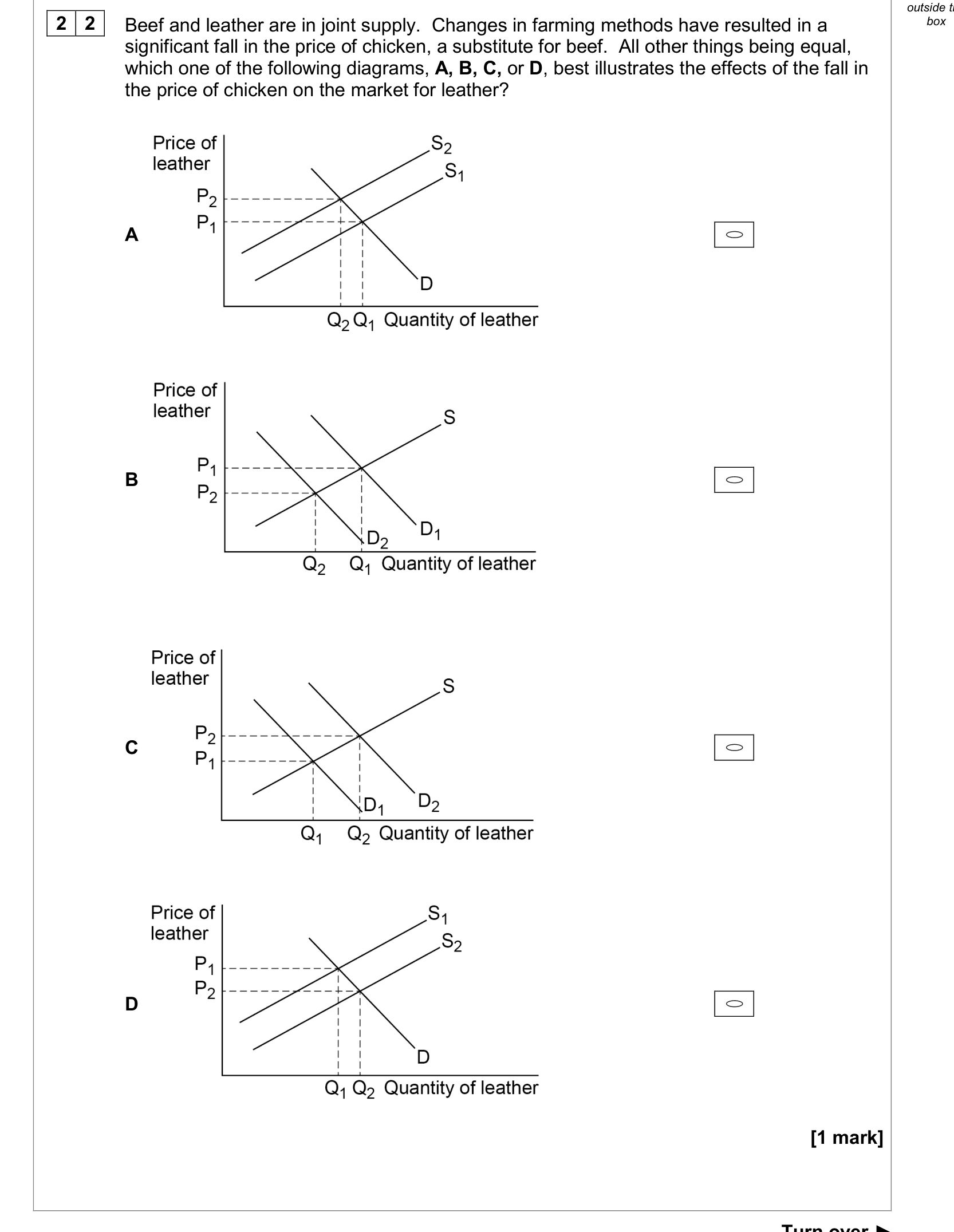
Beef and leather are in joint supply. Changes in farming methods have resulted in a significant fall in the price of chicken, a substitute for beef. All other things being equal, which one of the following diagrams, A, B, C, or D, best illustrates the effects of the fall in the price of chicken on the market for leather?
Answer: A.
Question 3
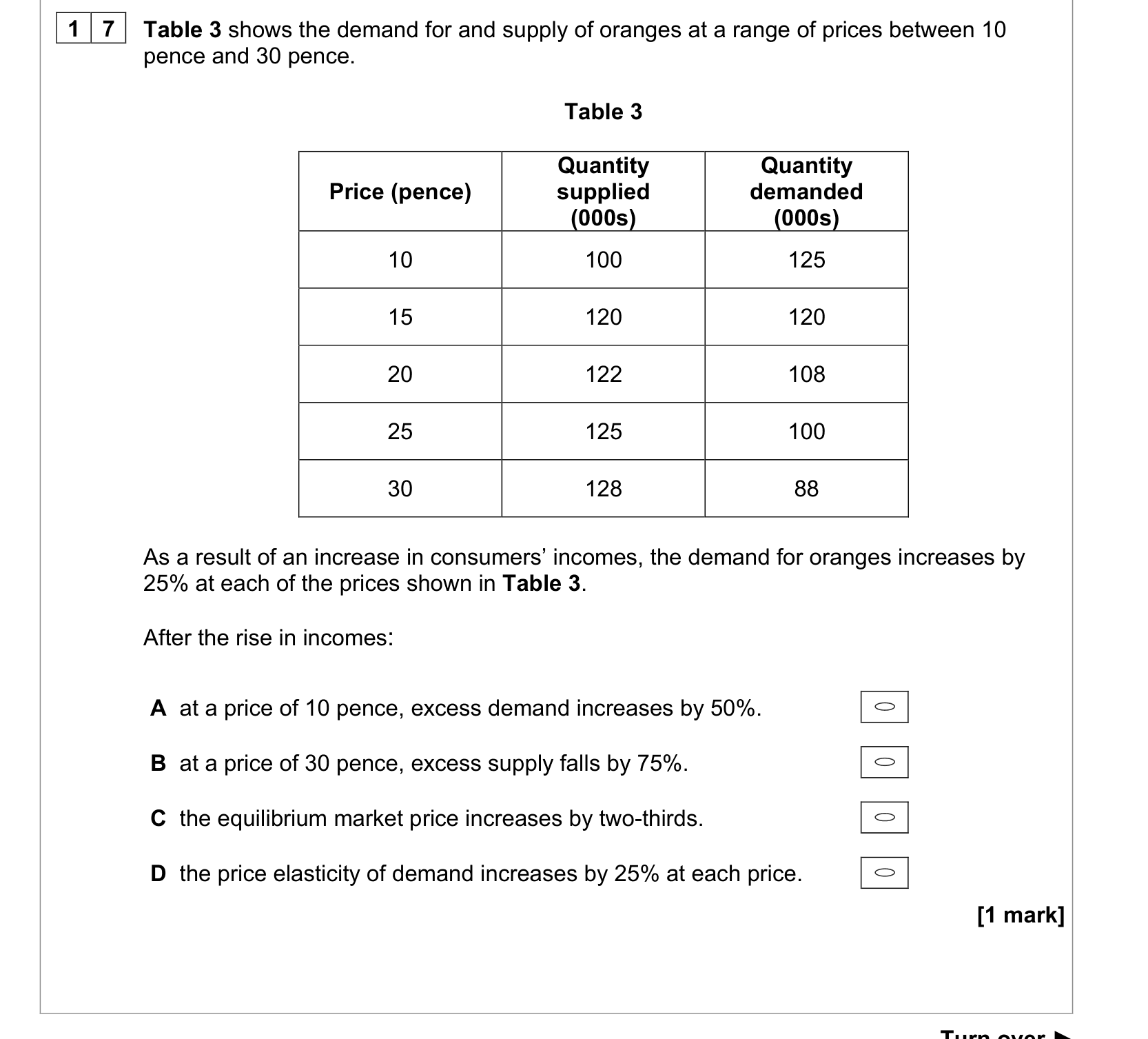
Table 3 shows the demand for and supply of oranges at a range of prices between 10 pence and 30 pence. Table 3 Price (pence) Quantity supplied (000s) Quantity demanded (000s) 10 100 125 15 120 120 20 122 108 25 125 100 30 128 88 As a result of an increase in consumers’ incomes, the demand for oranges increases by 25% at each of the prices shown in Table 3. After the rise in incomes:
Answer: C.
What the syllabus asks for on this topicSpecification points
Specification points
- Demand and supply, and the factors that shift them.
- Price, income and cross elasticities of demand (PED, YED, XED).
- Price elasticity of supply (PES).
Related AQA A-Level topics
Not the topic you were looking for? Describe what you are stuck on in your own words and we will take you to the notes that answer it.