Aggregate Demand and Aggregate Supply
Contents: 9 sections
Aggregate demand
Aggregate demand is total planned spending on domestic output at each price level, over a period of time.
AD = C + I + G + (X − M)
| Component | Key influences |
|---|---|
| Consumption (C) | Disposable income, consumer confidence, interest rates, wealth, credit availability |
| Investment (I) | Interest rates, business confidence, technology, corporate taxes, spare capacity |
| Government spending (G) | Fiscal policy, the stage of the economic cycle, political priorities |
| Net exports (X − M) | Exchange rates, foreign income, relative inflation, competitiveness |
C is the largest component in most economies, which is why consumer confidence matters so much to policymakers, and why interest-rate changes are transmitted so powerfully through households.
Two definitional traps that cost marks:
- Investment means spending by firms on capital goods, machinery, factories, and additions to inventories. Buying shares is a financial transaction, not investment in this sense.
- Government spending covers purchases of goods and services only. Transfer payments such as pensions and unemployment benefits are excluded, because nothing is produced in exchange. They affect AD only once the recipient spends them, which appears in C.
Why AD slopes downwards
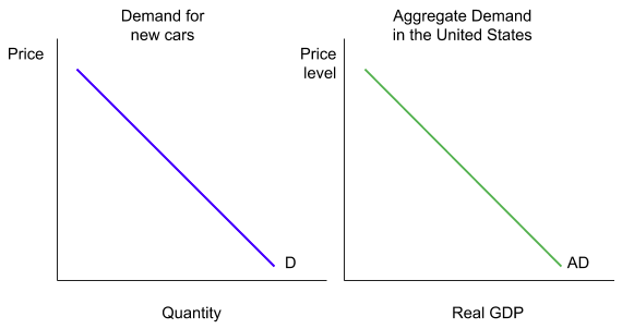
The reasons are not the same as for an individual demand curve, and examiners look for this distinction. A microeconomic demand curve slopes down because consumers substitute towards other goods; there is nothing to substitute towards when all prices fall together. Three separate mechanisms apply instead:
- Wealth effect. A lower price level raises the real value of money held by households, so they feel wealthier and spend more.
- Interest-rate effect. A lower price level reduces the demand for money; interest rates fall; investment and interest-sensitive consumption rise.
- International-trade effect. A lower domestic price level makes exports more competitive and imports less attractive, so net exports rise.
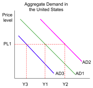
A change in the price level causes a movement along AD. A change in any component causes a shift.
Aggregate supply
SRAS slopes upward. In the short run money wages and some input prices are fixed by contract, so a higher price level widens profit margins and firms expand output. SRAS shifts with:
- wage rates and other input costs
- raw material and energy prices
- the exchange rate (through imported input costs)
- indirect taxes and subsidies on production
LRAS shows the economy's productive potential, what it can produce when all resources are fully and efficiently employed. It shifts only with the quantity or quality of factors of production: investment in capital, labour force growth, education and training, technology, and institutional improvements.
A rightward shift of LRAS is long-run economic growth, and it is the same event as an outward shift of the PPC. Being able to say that connects this topic to both the growth topic and the introductory unit.
The two views of LRAS
This disagreement is the heart of most 15-mark macro questions, and the examiner is looking for you to treat it as a genuine debate rather than pick one and forget the other.
- Monetarist / new-classical: LRAS is vertical at full-employment output (Yf). Markets clear, so the economy always returns to Yf. An increase in AD raises output only temporarily; in the long run it raises only the price level. The policy conclusion is that demand management cannot raise long-run output, only supply-side policy can.
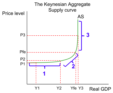
- Keynesian: LRAS has three sections, horizontal at low output (deep spare capacity, so extra demand raises output with no inflation), a curved intermediate section (bottlenecks appear, so output and prices both rise), and vertical at full capacity. The policy conclusion is that in a deep recession, demand management works and is necessary, because the economy can be stuck below full employment.
The disagreement is really about how quickly wages and prices adjust. New-classical economists think markets clear fast enough that the long run arrives soon; Keynesians argue nominal wages are sticky downwards, workers resist pay cuts and contracts are fixed, so an economy can sit below full employment for years. That is why the Keynesian case for intervention is strongest in a deep recession.
Macroeconomic equilibrium
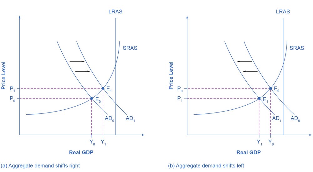
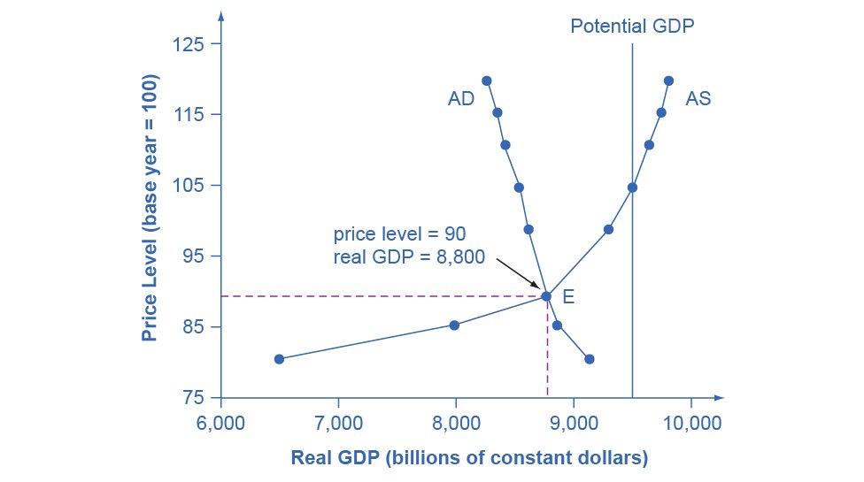
Equilibrium occurs where AD = AS, determining real output and the price level simultaneously.
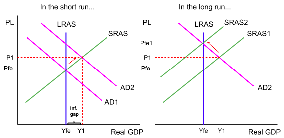
The figure shows the labelling standard an IB diagram needs: both curves named, both equilibria marked, and the price level and output read off each axis at each equilibrium.
Output gaps name the two disequilibrium positions:
- A deflationary (recessionary) gap exists when equilibrium output lies below full-employment output. Unemployment is above its natural rate and there is downward pressure on prices.
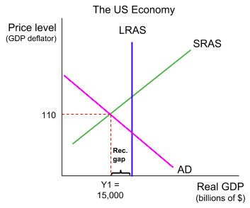
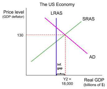
- An inflationary gap exists when equilibrium output lies above full-employment output. Unemployment is below its natural rate and there is upward pressure on prices.
The consequence of a demand increase depends entirely on where the economy is:
| Starting position | Effect of a rise in AD |
|---|---|
| Deep spare capacity (Keynesian horizontal section) | Output rises substantially; price level barely moves |
| Intermediate section | Output and price level both rise |
| At or near full capacity | Almost all the adjustment is in the price level: demand-pull inflation |
This is why "an increase in AD causes growth" is an incomplete answer. Whether it causes growth, inflation, or both is the analysis the question is asking for.
Demand-side and supply-side shocks
- Negative demand shock (collapse in confidence, export slump): AD shifts left → output falls, unemployment rises, price level falls or disinflates. This is a deflationary gap.
- Positive demand shock near capacity: AD shifts right → demand-pull inflation.
- Negative supply shock (oil price spike, harvest failure, currency depreciation raising import costs): SRAS shifts left → output falls AND the price level rises simultaneously. This is stagflation, and it is genuinely difficult for policymakers: demand management can fix one problem only by worsening the other.
The stagflation case is the strongest evaluation material in this topic, because it shows the limits of demand-side policy directly. Expansionary policy restores output but drives prices higher still; contractionary policy tames prices but deepens the fall in output. Neither instrument can address both, which is the argument for supply-side measures instead.
Real-world examples
The IB rewards real-world application, and this topic has three episodes worth being able to reference:
- The oil shocks of the 1970s are the classic negative supply shock. A sharp rise in oil prices raised costs across the economy, shifting SRAS left and producing high inflation alongside rising unemployment, the episode that gave stagflation its name and badly damaged confidence in demand management alone.
- The 2008 global financial crisis was a large negative demand shock. Collapsing confidence and a contraction in credit cut both consumption and investment, shifting AD sharply left and opening a deflationary gap in many economies. Governments responded with expansionary fiscal and monetary policy, which is the Keynesian prescription in action.
- The COVID-19 pandemic is useful precisely because it was both at once: lockdowns and supply-chain disruption shifted SRAS left, while lost incomes and collapsing confidence shifted AD left. That combination is why the output effect was unambiguous while the effect on the price level was not.
Use these to illustrate a mechanism you have already explained. An example dropped in without the analysis earns little; an example that shows the curve you just shifted actually shifting earns the application marks.
(HL) The multiplier
An initial injection into the circular flow produces a larger final change in national income, because one person's spending becomes another's income, which is then partly spent again.
k = 1 ÷ (1 − MPC)
equivalently k = 1 ÷ (MPS + MPT + MPM)
The second form is the one the IB prefers, because it names the three leakages explicitly:
- MPS: marginal propensity to save
- MPT: marginal propensity to tax
- MPM: marginal propensity to import
Note that MPC + MPS + MPT + MPM = 1: every extra unit of income is either spent domestically or leaks out of the circular flow in one of the three ways.
Worked calculation. An economy has MPS = 0.1, MPT = 0.2 and MPM = 0.1. The government increases spending by \$500 million.
k = 1 ÷ (0.1 + 0.2 + 0.1) = 1 ÷ 0.4 = 2.5
Change in national income = 2.5 × \$500m = \$1,250 million
So AD shifts right by the multiplied amount, \$1.25bn, not the initial \$500m. Shifting AD by the injection alone is a frequent lost mark.
What the multiplier does not tell you. It gives the size of the AD shift, not the rise in real output. How much becomes output rather than price level still depends on where the economy sits on the AS curve, near full capacity, most of a large AD shift becomes inflation.
Evaluation. The multiplier is smaller in an economy with high taxes, high import propensity or high saving, which is why the same stimulus does less in a very open economy: much of the spending leaks abroad as demand for imports. It also assumes spare capacity exists to respond.
Worked example
Suppose investment falls because business confidence collapses.
- Lower confidence
- firms postpone capital projects
- I falls
- AD shifts left from AD₁ to AD₂
- at the original price level there is now excess supply
- equilibrium real output falls from Y₁ to Y₂ and the price level falls from P₁ to P₂.
The split between output and prices depends on the AS curve. On the horizontal Keynesian section, nearly all of the fall shows up as lost output and rising cyclical unemployment, with little price adjustment. Near full employment, more of the adjustment falls on the price level.
There is a second round: lower output means lower incomes, which reduces consumption further. That is the multiplier, and mentioning it turns a good answer into a strong one, at HL, quantify it.
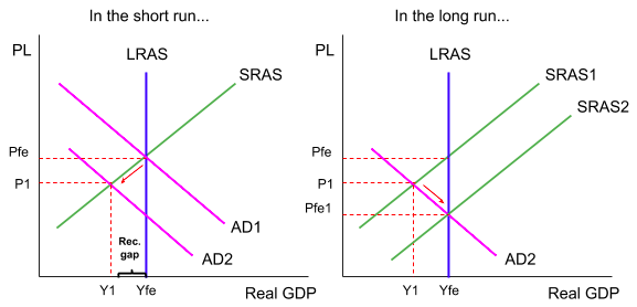
Then take it to the long run, which is where the two models diverge. On the new-classical view, the deflationary gap eventually closes itself: unemployment pushes nominal wages down, costs fall, SRAS shifts right, and output returns to Yf at a lower price level. On the Keynesian view, wages are sticky downwards, so the economy can remain stuck in the gap, which is precisely the case for government intervention. Naming both, and saying which you find more persuasive and why, is what a 15-mark answer needs.
Common exam mistakes
- Explaining the downward slope of AD using substitution, as if it were a microeconomic demand curve.
- Confusing a movement along AD (caused by the price level) with a shift (caused by a component).
- Counting transfer payments in G, or share purchases in I.
- Shifting LRAS for something that only affects SRAS, a wage rise changes costs, not productive potential.
- Treating the shape of LRAS as settled fact rather than a live disagreement.
- Labelling the axes "price" and "quantity" instead of price level and real output.
- Asserting that higher AD causes inflation without saying where the economy is on the AS curve.
- (HL) Shifting AD by the initial injection rather than the multiplied amount, or forgetting that taxes and imports are leakages too.
- Dropping in a real-world example without connecting it to a curve shift.
Exam technique
Label the axes price level and real output (real GDP); this is a common lost mark. Show the initial equilibrium, shift one curve at a time, and mark the new equilibrium with dotted lines to both axes.
State the cause of the shift, not just its direction: "AD shifts right because government spending rises" earns the analysis mark that "AD shifts right" does not.
Choose your AS model deliberately and say so. If the question is about a deep recession, the Keynesian diagram makes your argument visible; if it is about the long-run limits of demand management, the vertical LRAS does. Drawing one and arguing the other is a common self-inflicted contradiction.
For evaluation, the reliable routes are: where is the economy on the AS curve (this determines whether you get output or inflation), short run versus long run (the new-classical return to Yf), the size of the multiplier and its leakages, and time lags before policy takes effect.
Quick revision
- AD = C + I + G + (X − M); C is usually the largest component.
- G excludes transfer payments; I means firms' capital spending, not buying shares.
- AD slopes down via the wealth, interest-rate and international-trade effects, not substitution.
- SRAS shifts with input costs; LRAS shifts only with the quantity or quality of factors.
- LRAS: vertical at Yf (new-classical) or three-section (Keynesian); the dispute is about how fast wages adjust.
- Equilibrium at AD = AS sets real output and the price level together.
- Deflationary gap: output below Yf. Inflationary gap: above it.
- Whether a rise in AD gives growth or inflation depends on spare capacity.
- A negative supply shock raises prices and cuts output at once, stagflation.
- (HL) k = 1 ÷ (MPS + MPT + MPM); shift AD by the multiplied amount.
Check you have it
Cross-board concept practice · originally a CIE 9708 question, used here because the concept is the same. It is not IB Economics past-paper material.
Question 1
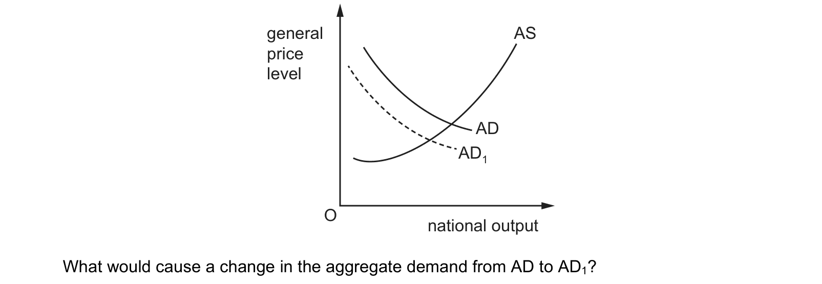
The diagram shows aggregate demand and aggregate supply curves for an economy. general price level O national output AS AD AD1 What would cause a change in the aggregate demand from AD to AD1?
Answer: C.
Cross-board concept practice · originally a CIE 9708 question, used here because the concept is the same. It is not IB Economics past-paper material.
Question 2
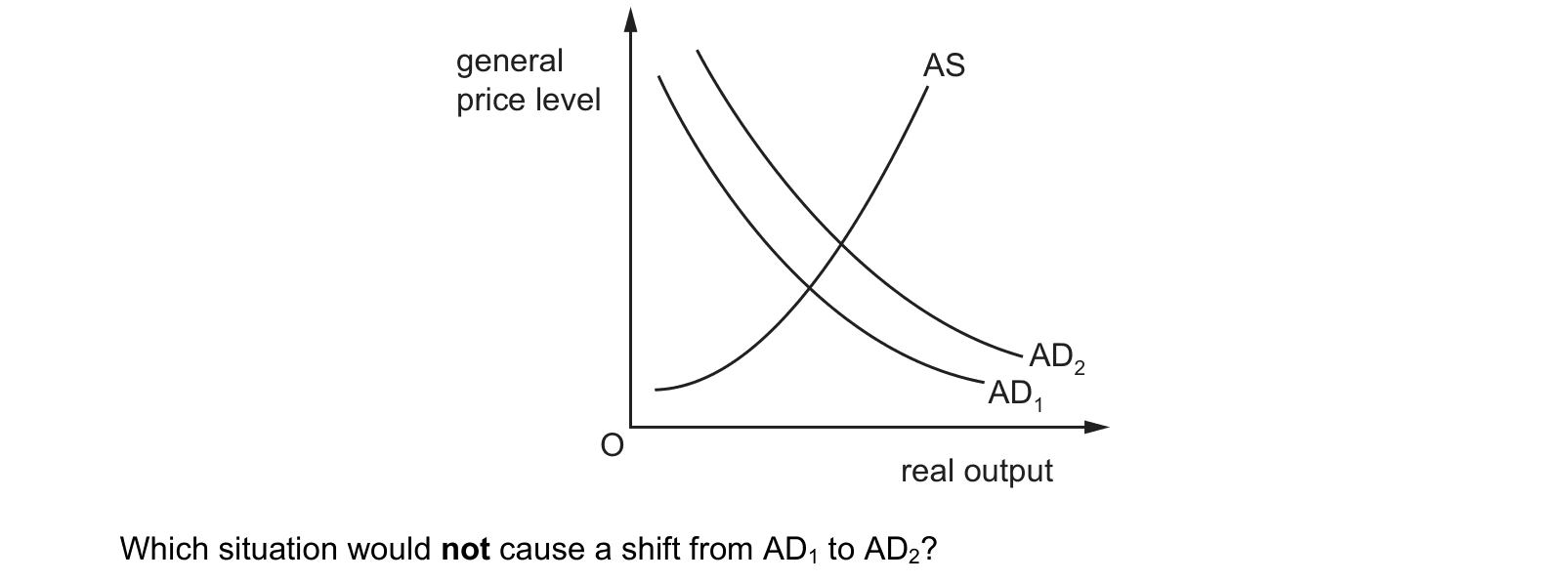
The diagram shows the aggregate demand (AD) and aggregate supply (AS) curves for an economy. general price level real output O AS AD2 AD1 Which situation would not cause a shift from AD1 to AD2?
Answer: A.
Cross-board concept practice · originally a CIE 9708 question, used here because the concept is the same. It is not IB Economics past-paper material.
Question 3
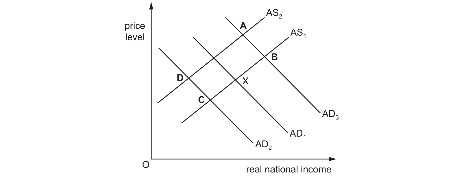
The government of a country plans to cut income tax rates. The initial equilibrium for the country is represented by point X on the diagram. Which new equilibrium point would an economist predict as the result?
Answer: B.
What the syllabus asks for on this topicSyllabus points
Syllabus points
- Define and explain the components of aggregate demand (AD).
- Explain the shape of, and shifts in, the AD curve.
- Distinguish short-run aggregate supply (SRAS) from long-run aggregate supply (LRAS).
- Explain equilibrium and the Keynesian versus monetarist/new-classical models.
- Analyse the effect of demand-side and supply-side shocks on output and the price level.
- (HL) Calculate and apply the Keynesian multiplier.
This is the model the rest of macroeconomics runs on. Fiscal policy, monetary policy and supply-side policy all end by shifting a curve on this diagram, so anything vague here becomes vague in three other topics as well.
Related IB Economics topics
Not the topic you were looking for? Describe what you are stuck on in your own words and we will take you to the notes that answer it.