Fiscal Policy
Contents: 12 sections
What fiscal policy is
Fiscal policy is the use of government spending and taxation to influence aggregate demand and achieve macroeconomic objectives. It is set by the government, which is the key distinction from monetary policy, set by the central bank.
Sources of government revenue: direct taxes (income tax, corporation tax), indirect taxes (VAT, excise duties), national insurance or social contributions, and revenue from state-owned assets and privatisation.
- Direct taxes are levied on income or wealth and paid straight to the government by the person or firm liable. They are the main tool for equity, because they can be made progressive.
- Indirect taxes are levied on spending and collected by sellers. They tend to be regressive, since lower-income households spend a larger share of their income.
Government expenditure falls into three useful categories:
- Current spending: day-to-day running costs: public sector wages, medicines, fuel.
- Capital spending: investment in infrastructure, schools, hospitals. This is the category that also raises potential output.
- Transfer payments: pensions, unemployment benefits. These are not part of G in AD, because no output is produced in exchange; they raise AD indirectly by raising disposable income and therefore consumption.
The transfer-payment point is a common lost mark. Increased benefits do not appear in G; they work through C.
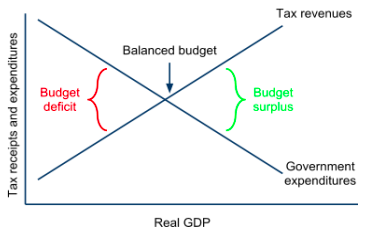
The budget position
| Position | Meaning |
|---|---|
| Budget deficit | Government spending exceeds revenue in a period |
| Budget surplus | Revenue exceeds spending |
| Balanced budget | The two are equal |
| National debt | The accumulated stock of past deficits |
Deficit and debt are a flow and a stock, and confusing them is a frequent error. A government can reduce its deficit every year and still see its debt rise, because any deficit adds to the stock.
Judge debt as a ratio, not a level. Sustainability is measured by debt as a percentage of GDP, because GDP is the income out of which debt is serviced. It follows that if nominal GDP grows faster than debt, the ratio falls even while the debt itself rises.
Cyclical versus structural. The budget balance moves with the economic cycle even when no policy has changed, because revenue and benefit spending respond automatically to income. The cyclical component is caused by the economy's position; the structural component is what the balance would be at full employment, and it is the part that reflects actual policy decisions. A deficit widening in a recession is therefore not proof that policy has loosened.
How fiscal policy affects AD
Recall AD = C + I + G + (X − M).
- Government spending changes G directly, the most immediate channel.
- Income tax changes disposable income, and therefore C.
- Corporation tax changes retained profit and expected returns, and therefore I.
- Indirect taxes change real disposable income and prices, affecting C.
Written as a chain:
- The government raises capital spending on infrastructure
- G rises
- AD shifts right
- firms raise output to meet the demand
- employment and incomes rise
- those higher incomes are partly re-spent
- consumption rises further.
That final step is the multiplier, and it means the eventual increase in national income exceeds the initial injection. The multiplier is larger when households spend a high proportion of extra income domestically, and smaller when much of it leaks into saving, taxation or imports.
(HL) Quantifying the injection
k = 1 ÷ (MPS + MPT + MPM)
A government raises spending by \$400 million in an economy where MPS = 0.15, MPT = 0.20 and MPM = 0.15.
k = 1 ÷ (0.15 + 0.20 + 0.15) = 1 ÷ 0.5 = 2
Change in national income = 2 × \$400m = \$800 million
So AD shifts right by \$800m, not \$400m. Two points follow that examiners look for:
- The multiplier tells you the size of the AD shift, not the rise in real output. How much becomes output rather than price level depends on where the economy sits on the AS curve.
- A more open or more heavily taxed economy has a smaller multiplier, because more of each round leaks away. The same stimulus therefore achieves less in a very open economy, a strong comparative evaluation point.
Expansionary versus contractionary
| Stance | Action | Aim | Risk |
|---|---|---|---|
| Expansionary | Raise G, cut taxes | Raise AD in a recession; cut cyclical unemployment | Inflation near capacity; larger deficit and debt |
| Contractionary | Cut G, raise taxes | Reduce AD to control demand-pull inflation; improve the budget | Slower growth, higher unemployment |
Watch the vocabulary trap: "expansionary" describes the effect on AD, not on the budget. An expansionary policy worsens the budget balance. The two move in opposite directions.
Beyond aggregate demand
The IB expects fiscal policy to be understood as more than demand management. It has three roles:
- Influencing AD: the short-run stabilisation role above.
- Promoting equity: progressive income taxes and transfer payments redistribute from higher to lower incomes, which is the main instrument any government has for reducing inequality.
- Supporting potential output: spending on infrastructure, education, healthcare and research raises the quantity and quality of factors of production, shifting LRAS right. This is where fiscal policy overlaps with supply-side policy, and noticing that overlap is a genuine discriminator.
That third role is why capital spending is treated differently from current spending in evaluation: borrowing to build something that raises future output can service itself, while borrowing to fund current consumption cannot.
Automatic stabilisers
Some fiscal effects operate without any policy decision, which is why they matter:
- In a downturn, incomes fall so tax revenue falls automatically, while unemployment benefit spending rises automatically. Both cushion the fall in AD.
- In a boom, tax revenue rises and benefit spending falls, dampening the expansion.
Automatic stabilisers reduce the amplitude of the business cycle with no time lag at all, a genuine advantage over discretionary policy, and a strong point to make in evaluation. They are stronger where income taxes are progressive and welfare systems generous, which links the stabilisation and equity roles together.
Evaluation
Strengths
- Targeted. Unlike interest rates, which affect the whole economy uniformly, spending can be directed at specific regions, industries or groups.
- Effective at the zero lower bound. When interest rates are already near zero and monetary policy is in a liquidity trap, fiscal policy still works, the central argument for fiscal stimulus after 2008.
- Capital spending raises potential output too, shifting LRAS right as well as AD, so it can deliver both actual and potential growth.
- Automatic stabilisers act instantly and without political decision.
- Directly addresses equity, which monetary policy cannot.
Limitations
- Time lags. The recognition lag (identifying the problem), the decision lag (budgets are typically annual and politically contested), and the implementation lag (infrastructure takes years) together mean the stimulus can arrive after the recession has ended, making it pro-cyclical.
- Crowding out. Financing a deficit by borrowing raises demand for loanable funds, pushing up interest rates and potentially displacing private investment.
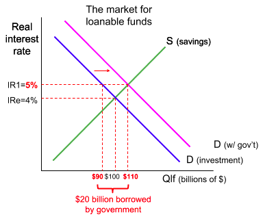 How serious this is depends on the state of the economy: with substantial spare capacity and idle savings, crowding out is likely to be small.
- Political constraints. Raising taxes and cutting spending are unpopular, so contractionary policy is systematically harder to enact than expansionary. This creates a deficit bias over the cycle.
- Debt sustainability. Persistent deficits raise debt, interest payments consume a growing share of the budget, and at some point credit ratings and borrowing costs deteriorate.
- Uncertainty about the multiplier, which varies with the state of the economy and the leakages present.
- Ineffective against cost-push inflation, exactly as monetary policy is.
Real-world examples
- The post-2008 stimulus programmes are the standard case for fiscal policy at the zero lower bound: with interest rates already near zero across the major economies, governments turned to spending increases and tax cuts because monetary policy had run out of conventional room.
- The austerity programmes that followed in parts of Europe are the counter-case, and the live disagreement: whether consolidating budgets while output was still below potential deepened and prolonged the downturn, or was necessary to keep borrowing costs sustainable. A question asking you to evaluate fiscal policy is inviting exactly this argument.
- The COVID-19 support schemes show the targeting advantage directly, wage subsidies and grants aimed at the specific households and firms losing income, which no interest-rate change could have replicated.
Worked example
An economy is in recession: unemployment is 9%, output is below potential, and the central bank has already cut rates to near zero. The government announces a large infrastructure programme.
- G rises
- AD shifts right from AD₁ to AD₂
- with spare capacity, firms respond by raising real output rather than prices
- unemployment falls
- higher incomes raise consumption through the multiplier, shifting AD further right.
Why fiscal rather than monetary here? Monetary policy is at the zero lower bound and cannot cut further. Fiscal policy still has traction. That diagnostic sentence is worth more than a list of fiscal advantages.
The qualifications. Infrastructure has a long implementation lag, so the spending may arrive after recovery has begun. It must be financed by borrowing, adding to debt. But because the economy has spare capacity and private investment is weak, crowding out is likely to be limited, and since it is capital spending, it raises potential output as well, shifting LRAS right in the long run.
A judgement, not a list. The strongest conclusion is conditional: fiscal expansion is well suited to this case, deep spare capacity, monetary policy exhausted, and spending that adds to capacity, but the same policy near full employment would be largely inflationary and would crowd out private investment far more heavily. Saying what the answer depends on is what separates the top band.
Common exam mistakes
- Confusing fiscal policy (government, tax and spending) with monetary policy (central bank, interest rates).
- Counting transfer payments as part of G.
- Confusing the budget deficit (a flow) with national debt (a stock).
- Assuming a widening deficit proves policy has loosened, when the cause may be cyclical.
- Asserting crowding out will occur without considering spare capacity.
- Ignoring time lags, which are far longer for fiscal than for monetary policy.
- Forgetting that capital spending affects both AD and LRAS.
- (HL) Shifting AD by the initial injection rather than the multiplied amount.
Exam technique
Trace the chain explicitly, policy → the AD component affected → AD shift → output, employment and price level, and name the multiplier at the end.
Draw AD–AS with axes labelled price level and real output. Where the question concerns capital spending, consider showing LRAS shifting right as well; that dual effect is a genuine discriminator at the top band.
For evaluation, the strongest routes are: spare capacity (which decides whether you get output or inflation), time lags, crowding out and whether it actually binds, debt sustainability, the size of the multiplier, and a comparison with monetary policy, which acts faster but is blunt and can be trapped at the zero bound. End with a conditional judgement.
Quick revision
- Fiscal policy = government spending and taxation; set by government, not the central bank.
- Direct taxes fall on income and can be progressive; indirect taxes fall on spending and tend to be regressive.
- Transfer payments raise AD through C, not G.
- Deficit is a flow; national debt is the accumulated stock, judged as a share of GDP.
- Cyclical deficits move with the economy; structural deficits reflect policy.
- Expansionary: raise G, cut taxes. Contractionary: the reverse.
- Three roles: influence AD, promote equity, raise potential output.
- Automatic stabilisers work instantly, with no policy lag.
- (HL) k = 1 ÷ (MPS + MPT + MPM); shift AD by the multiplied amount.
- Strengths: targeted, works at the zero lower bound, capital spending raises LRAS, addresses equity.
- Limits: long lags, crowding out (depends on capacity), political bias, debt.
Check you have it
Cross-board concept practice · originally a CIE 9708 question, used here because the concept is the same. It is not IB Economics past-paper material.
Question 1
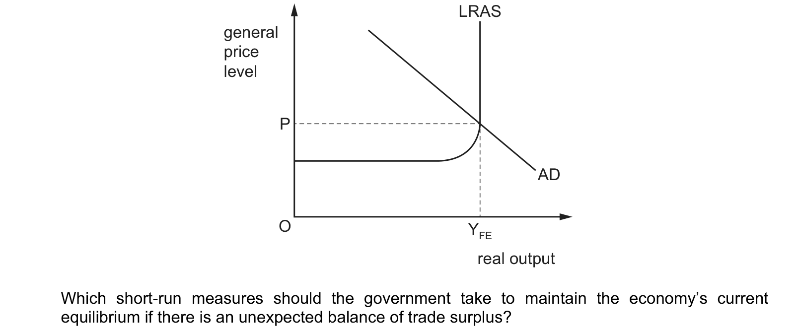
The diagram shows an economy at full employment equilibrium. general price level real output O LRAS AD P YFE Which short-run measures should the government take to maintain the economy’s current equilibrium if there is an unexpected balance of trade surplus?
Answer: B.
To hold the current equilibrium the government must offset that injection with an equal withdrawal, which means a CONTRACTIONARY fiscal stance: higher direct taxation with spending unchanged, running a budget surplus: B.
- A raises spending and taxation together. A balanced-budget change is mildly expansionary, not contractionary, because government spending injects the full amount while higher taxes cut consumption by less than the full amount, part comes out of saving.
- C and D are both expansionary, so each adds to the very pressure that needs offsetting.
Cross-board concept practice · originally a CIE 9708 question, used here because the concept is the same. It is not IB Economics past-paper material.
Question 2
Why are higher interest rates together with increased taxation on expenditure likely to cause domestic deflation?
Answer: B.
Cross-board concept practice · originally a CIE 9708 question, used here because the concept is the same. It is not IB Economics past-paper material.
Question 3
What is an example of contractionary fiscal policy?
Answer: B.
What the syllabus asks for on this topicSyllabus points
Syllabus points
- Define fiscal policy and identify the sources of government revenue and expenditure.
- Explain how fiscal policy is used to influence aggregate demand.
- Distinguish expansionary from contractionary fiscal policy.
- Explain the role of fiscal policy in promoting equity and potential output.
- Evaluate the strengths and limitations of fiscal policy.
- (HL) Apply the multiplier to a fiscal injection.
Related IB Economics topics
Not the topic you were looking for? Describe what you are stuck on in your own words and we will take you to the notes that answer it.