Elasticity of Supply (PES)
Contents: 9 sections
Price elasticity of supply
PES measures how responsive quantity supplied is to a change in the good's price.
PES = percentage change in quantity supplied ÷ percentage change in price
Because the supply curve slopes upward, price and quantity move in the same direction, so PES is normally positive. This is the mirror image of PED, which is negative, and a quick way to check you have not muddled the two.
| Value | Name | What it means |
|---|---|---|
| PES > 1 | Elastic | Producers respond more than proportionately |
| PES < 1 | Inelastic | Producers respond less than proportionately |
| PES = 1 | Unit elastic | Proportional response |
| PES = 0 | Perfectly inelastic | Quantity fixed regardless of price (vertical curve) |
| PES = ∞ | Perfectly elastic | Any quantity supplied at one price (horizontal curve) |
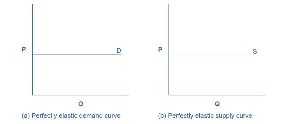
Reading PES off the diagram
A useful result that examiners test directly, because it can be answered from a sketch with no calculation at all. For a straight-line supply curve:
| Where the curve cuts | PES |
|---|---|
| Through the origin | Exactly 1 at every point |
| The price axis (positive intercept on P) | Greater than 1: elastic |
| The quantity axis (positive intercept on Q) | Less than 1: inelastic |
Note this is unlike demand, where elasticity varies along a single straight line. A supply curve through the origin has PES = 1 everywhere along it, however steep it is drawn, so steepness alone does not tell you elasticity.
Key definitions
| Term | Exam-ready definition |
|---|---|
| PES | Responsiveness of quantity supplied to a change in the good's price. |
| Spare capacity | Unused productive capability allowing output to rise quickly. |
| Perishability | How quickly a good deteriorates, limiting the ability to store it. |
| Momentary supply | Supply immediately after a price change, before any adjustment. |
Determinants of PES
Time is the dominant determinant, and it deserves its own treatment. Economists distinguish three periods:
- Momentary period. Supply is effectively fixed, perfectly inelastic. A farmer whose crop is already harvested cannot produce more today at any price.
- Short run. At least one factor is fixed. Output can be raised somewhat by using variable factors more intensively, overtime, extra shifts, so supply is inelastic but not perfectly so.
- Long run. All factors are variable. Firms can build capacity and new firms can enter, so supply is far more elastic.
The other determinants:
- Spare capacity. A firm operating below full capacity can raise output quickly, making supply elastic. A firm at full capacity cannot, whatever the price.
- Stocks (inventories). Goods that can be stored allow firms to release stock immediately when price rises, elastic supply. This is why perishability matters so much.
- Mobility of factors of production. If labour and capital can be switched easily between uses, supply is elastic. Highly specialised equipment or skills make it inelastic.
- Ease of entry. Low barriers to entry mean new firms arrive when price rises, raising market supply.
- Length of the production process. Goods with long lead times, timber, mined ore, tree crops, aircraft, have inelastic supply because production cannot be accelerated.
Primary commodities versus manufactured goods
This comparison is explicitly on the syllabus and appears constantly in development questions.
| Primary commodities | Manufactured goods | |
|---|---|---|
| PES | Low (inelastic) | Higher (elastic) |
| Why | Long growing or extraction periods; land is fixed; output depends on weather; crops are perishable | Production can be scaled with shifts and capacity; inputs are mobile; goods are storable |
Why this matters. Primary products tend to have both inelastic supply and inelastic demand. When either curve shifts, a bad harvest, a demand shock, the adjustment falls almost entirely on price rather than quantity. The result is volatile prices and volatile incomes for primary producers.
That volatility is a serious development problem: it makes farm incomes unpredictable, makes government revenue unpredictable in commodity-dependent economies, and makes planning and investment harder. It is the standard economic justification for buffer stock schemes, price supports and diversification strategies, and it is the reason economies dependent on primary exports are urged to diversify into manufacturing.
Buffer stock schemes deserve a sentence of their own, because the mechanism is examinable. The agency sets a price band: when the market price falls towards the floor it buys and stores the surplus, and when the price rises towards the ceiling it releases stock from store. In principle this stabilises both prices and incomes. In practice the schemes have often failed, storage is expensive, perishable goods cannot be held indefinitely, and if the floor is set above the long-run equilibrium the agency accumulates stock it can never sell and eventually runs out of money. That two-sided treatment is what an evaluation question wants.
Worked example
Calculating. The price of wheat rises from \$200 to \$240 per tonne, and quantity supplied rises from 50,000 to 55,000 tonnes.
%ΔQs = 5,000 ÷ 50,000 × 100 = 10%
%ΔP = 40 ÷ 200 × 100 = 20%
PES = 10% ÷ 20% = 0.5
PES is less than 1, so supply is inelastic: farmers cannot expand output much within a growing season, because land is fixed and the crop cycle cannot be accelerated.
Interpreting. Because supply is inelastic, a rise in demand for wheat would push the price up sharply while quantity barely moved. Over several seasons, however, farmers can plant more land and PES rises, so the same demand increase produces more output and less price rise in the long run. Saying that explicitly is what turns a calculation into analysis.
Apply it to a policy. Suppose the government subsidises wheat production to raise output.
- With PES = 0.5, supply is inelastic
- the rightward shift produces a small increase in quantity and a large fall in price
- most of the subsidy ends up raising producers' effective revenue per tonne rather than the tonnage grown.
If the policy aim was food security through greater output; that is close to a failure, and PES is the reason. The same subsidy applied to a manufactured good with elastic supply would deliver far more extra output per dollar spent. PES is the hidden variable that decides whether a supply-side policy achieves quantity or merely price.
Common exam mistakes
- Giving PES a negative sign. It is normally positive, because supply slopes upward.
- Confusing PES with PED, or applying the "total revenue test" to PES, that test belongs to PED.
- Ignoring the time period. "Supply is inelastic" is incomplete without saying over what horizon.
- Judging elasticity from the steepness of a straight-line supply curve rather than from where it cuts an axis.
- Treating spare capacity and stocks as the same thing. Capacity is about the ability to produce more; stocks are about releasing what already exists.
- Calculating PES correctly and never interpreting it.
- Saying primary products have inelastic supply without explaining why (fixed land, long production periods, weather).
- Presenting buffer stocks as straightforwardly effective.
Exam technique
Calculate, interpret, apply. Show the formula, substitute, compute, then state elastic or inelastic and say what it means for the market, price volatility, producer income, or the effectiveness of a policy.
PES is often the hidden variable in policy questions. When a government subsidises a good, how much output actually rises depends on PES; if supply is inelastic, most of the subsidy raises price rather than quantity. The same logic applies to any demand-side stimulus in a market with capacity constraints.
If a diagram is given rather than data, read the elasticity from where the supply curve cuts an axis, not from how steep it looks.
For evaluation, the strongest routes are the time frame (supply is more elastic in the long run, so short-run and long-run answers differ), spare capacity, and whether the elasticity estimate is reliable.
Quick revision
- PES = %ΔQs ÷ %ΔP; normally positive; >1 elastic, <1 inelastic.
- A straight-line supply curve through the origin has PES = 1 at every point.
- Cutting the price axis → elastic; cutting the quantity axis → inelastic.
- Time is the main determinant: momentary (fixed) → short run (limited) → long run (elastic).
- Also: spare capacity, stocks, factor mobility, ease of entry, length of production.
- Primary commodities have low PES; manufactures have higher PES.
- Inelastic supply plus inelastic demand → volatile prices and volatile producer incomes.
- Buffer stocks aim to stabilise this but are costly and fail if the floor is set too high.
- Inelastic supply means demand shocks, and subsidies, hit price, not quantity.
Check you have it
Cross-board concept practice · originally a CIE 9708 question, used here because the concept is the same. It is not IB Economics past-paper material.
Question 1
The diagram shows the supply curve of a product. The government imposes a specific indirect tax of $5 on the product. How will the price elasticity of supply of the product change?
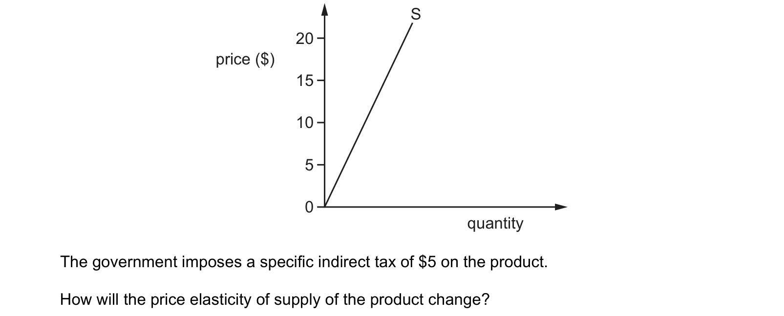
Answer: D.
Cross-board concept practice · originally a CIE 9708 question, used here because the concept is the same. It is not IB Economics past-paper material.
Question 2
The diagram shows two linear supply curves labelled S1 and S2, where S2 is a 45° line. Which statement about the price elasticity of supply is correct?
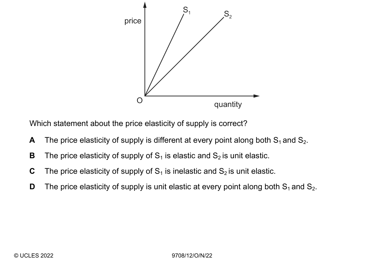
Answer: D.
Cross-board concept practice · originally a CIE 9708 question, used here because the concept is the same. It is not IB Economics past-paper material.
Question 3
The diagram shows the supply curve for bananas. What is the price elasticity of supply when there is a rise in price from $5 to $6?
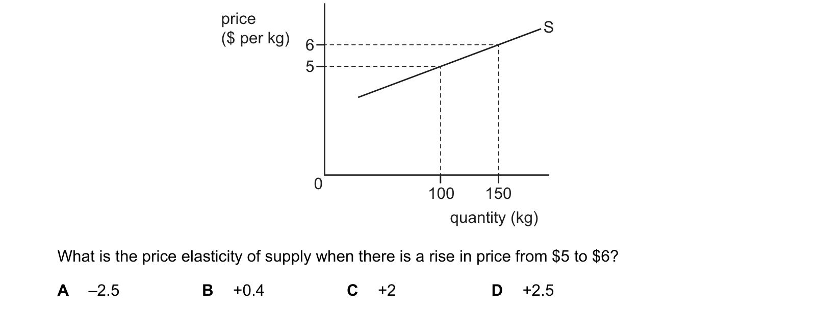
Answer: D.
What the syllabus asks for on this topicSyllabus points
Syllabus points
- Calculate and interpret price elasticity of supply (PES).
- Explain the determinants of PES.
- Apply PES to primary commodities versus manufactured goods.
Related IB Economics topics
Not the topic you were looking for? Describe what you are stuck on in your own words and we will take you to the notes that answer it.