Supply
Contents: 11 sections
The law of supply
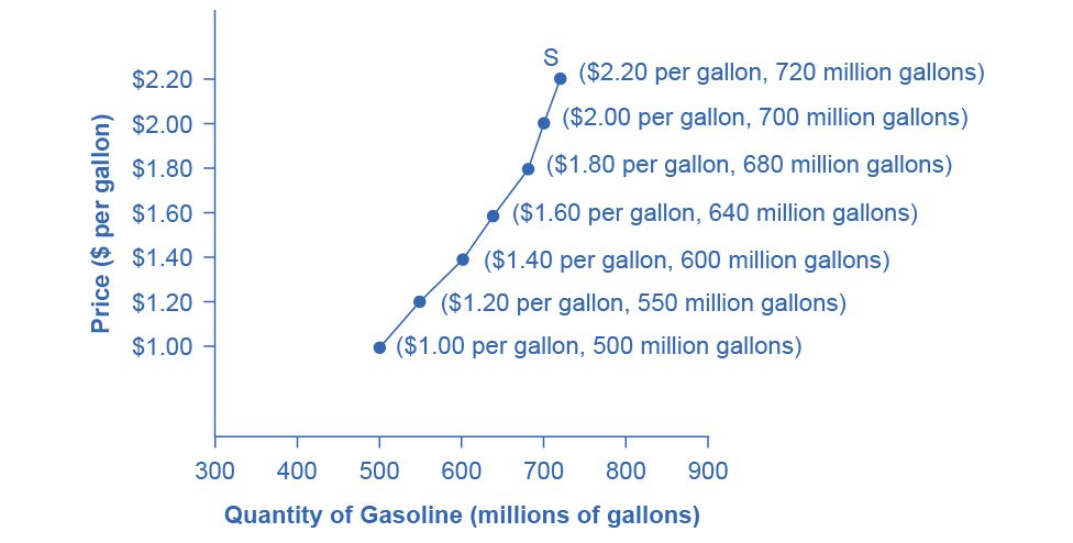
Supply is the quantity of a good producers are willing and able to sell at each price over a given period of time.
The law of supply states that, ceteris paribus, as price rises quantity supplied rises. The supply curve slopes upwards.
Two reasons explain the positive slope:
- The profit motive. A higher price, with costs unchanged, widens the margin on each unit. Existing firms expand output, and over time new firms are attracted into the market.
- Rising marginal costs. As a firm pushes output up in the short run, it adds variable factors to a fixed factor, so productivity per extra unit eventually falls and the cost of producing each additional unit rises. Firms therefore need a higher price to make that extra, more expensive unit worth producing.
The second reason is the more rigorous one, and mentioning diminishing returns is what separates a strong explanation from a superficial one.
It also gives the supply curve a second reading, mirroring demand: the supply curve is the marginal cost curve. Its height at any quantity is the cost of producing that unit, which is why the area above it and below the price is producer surplus, and why price equalling marginal cost at equilibrium is the definition of allocative efficiency.
Key definitions
| Term | Exam-ready definition |
|---|---|
| Supply | The quantity producers are willing and able to sell at each price. |
| Law of supply | As price rises, quantity supplied rises, ceteris paribus. |
| Movement along | A change in quantity supplied caused only by the good's own price. |
| Shift | A change in supply at every price caused by a non-price factor. |
| Marginal cost | The cost of producing one more unit. |
Movement along versus a shift
The same rule as demand, and it is tested just as often:
- A change in the good's own price
- a movement along the supply curve, a change in quantity supplied.
- A change in any other factor
- a shift of the whole curve, a change in supply.
The trap examiners set most often is an indirect tax. A tax is not a price change from the producer's point of view; it is a cost change, so it shifts supply left. Students who treat it as a movement along, or worse as a demand-side change, lose the analysis marks for the whole question.
Non-price determinants of supply
- Costs of production: wages, raw materials, energy, rent. Higher costs shift supply left.
- Technology: improvements raise productivity and shift supply right. Technological regress is rare, so this shift is usually one-directional over time.
- Indirect taxes: raise unit costs, shifting supply left by the amount of the tax. Subsidies shift it right.
- Prices of related goods: if a farmer can grow wheat or barley, a rise in the barley price draws land away from wheat, shifting wheat supply left (competitive supply). Where goods are produced together, such as beef and leather, more of one means more of the other (joint supply).
- Number of firms: more producers shift market supply right; firms exiting shift it left.
- Expectations and shocks: weather, natural disasters, conflict, supply-chain disruption, and expectations of future prices.
(HL) The linear supply function
Qs = c + dP
where d measures how strongly quantity supplied responds to price. The constant c is usually negative, which has a real meaning rather than being an algebraic oddity: below a certain price, no firm covers its costs and quantity supplied is zero.
Worked example. Qs = −40 + 4P.
| Price | Quantity supplied |
|---|---|
| \$10 | 0 |
| \$20 | 40 |
| \$30 | 80 |
| \$40 | 120 |
Setting Qs = 0 gives −40 + 4P = 0, so P = 10: the lowest price at which anything is supplied at all. Below \$10 the curve does not exist, quantity supplied is zero, not negative, which is why a plotted supply curve starts at the price axis rather than continuing below it.
What changes what. A change in c shifts the whole curve, the effect of a cost change, a tax, a subsidy or a change in the number of firms. A change in d rotates it. A change in P alone moves you along it.
Elasticity, briefly
How far quantity responds to price is the subject of 2.5, but one point belongs here: supply is almost always more elastic in the long run, because in the short run at least one factor is fixed. A firm cannot build a factory in a week, so a price rise this month produces a much smaller output response than the same rise sustained over years. This is why short-run shocks to commodity markets move prices so violently and quantities so little.
Individual and market supply
Market supply is the horizontal sum of all individual firms' supply curves: at each price, add the quantities every firm would offer. Entry and exit therefore shift market supply even when no existing firm changes its behaviour.
Worked example
A government grants a per-unit subsidy to solar-panel manufacturers.
- The subsidy reduces the effective cost of producing each panel
- at every price firms are willing to supply more
- the supply curve shifts right, from S₁ to S₂, vertically downwards by the amount of the subsidy per unit
- at the original price there is now excess supply
- price falls from P₁ to P₂ and the quantity traded rises from Q₁ to Q₂.
Two points worth adding, because they turn description into analysis:
- Who gains depends on elasticity. If demand is inelastic, most of the subsidy passes to producers as a higher effective price; if demand is elastic, more of it reaches consumers as a lower price.
- The subsidy has an opportunity cost. It is funded from taxation or borrowing, so the money is unavailable for other uses, the standard evaluation point on any subsidy question.
And the justification, which the strongest answers reach for. A subsidy on solar panels is not simply industrial favouritism: solar generation produces a positive externality by displacing emissions, so the free market under-provides it. That reframes the policy as correcting a market failure rather than distorting a working market, and it connects this topic directly to 2.8.
Second worked example: a per-unit tax
A government imposes a \$5 per-unit tax on a good.
- Each unit now costs the firm \$5 more to bring to market
- supply shifts vertically upwards by exactly \$5
- the new equilibrium has a higher price and lower quantity.
The precision matters: the vertical gap between S₁ and S₂ is \$5 at every quantity, which is what makes it a parallel shift for a specific per-unit tax. Note also that the price consumers pay does not rise by the full \$5 unless demand is perfectly inelastic, the burden is shared, and how it splits depends on the relative elasticities. Drawing the shift as \$5 and then claiming the price rose by \$5 is a common contradiction between diagram and prose.
Common exam mistakes
- Confusing a shift (cost, technology, tax) with a movement along (own-price change).
- Treating an indirect tax as a demand-side change. It raises firms' costs and shifts supply.
- Writing that a price rise "increases supply", it increases quantity supplied.
- Shifting supply for a change in consumer incomes or tastes, which are demand factors.
- Unlabelled diagrams, or shifting the curve without marking the new equilibrium.
- Forgetting that a per-unit tax shifts supply vertically by the tax amount, not by an arbitrary distance.
- Claiming price rises by the full amount of a per-unit tax.
- (HL) Extending the supply curve below the price at which Qs = 0, into negative quantities.
Exam technique
Name the exact determinant causing the shift and its direction, "supply shifts left because energy costs rose" rather than "supply shifts left".
When a tax or subsidy shifts supply, show the vertical distance between the two curves as the tax or subsidy per unit, and be ready to discuss incidence: who ultimately bears the burden or captures the benefit depends on the relative elasticities of demand and supply.
Given a supply function, solve for the price at which Qs = 0 before plotting. That is where the curve meets the price axis, and it anchors the whole line.
For evaluation, consider the time frame (supply is far more elastic in the long run, once firms can vary all factors), the size of the cost change, and whether firms have spare capacity to respond at all.
Quick revision
- Supply curve slopes up: profit motive plus rising marginal costs from diminishing returns.
- The supply curve is the marginal cost curve; its area under the price is producer surplus.
- Own price → movement along (quantity supplied). Anything else → shift (supply).
- Determinants: costs, technology, taxes and subsidies, related goods, number of firms, shocks.
- An indirect tax shifts supply left vertically by the tax per unit; a subsidy shifts it right.
- Price does not rise by the full tax unless demand is perfectly inelastic.
- Competitive supply pulls resources between goods; joint supply produces them together.
- Supply is more elastic in the long run.
- (HL) Qs = c + dP, with c usually negative; solve Qs = 0 for the minimum supply price.
Check you have it
Cross-board concept practice · originally a CIE 9708 question, used here because the concept is the same. It is not IB Economics past-paper material.
Question 1
The diagram shows an industry’s demand and supply curves. The industry increases supply from S1 to S2. Which area shows the total gain in society’s economic welfare?
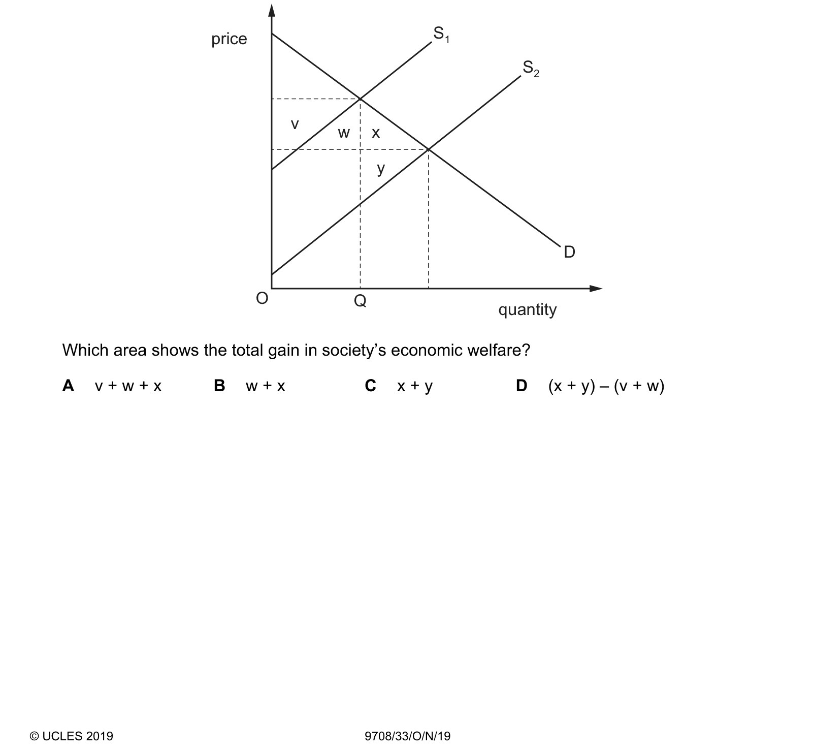
Answer: C.
Cross-board concept practice · originally a CIE 9708 question, used here because the concept is the same. It is not IB Economics past-paper material.
Question 2
In the diagram, Q1 is the quantity produced of a good as the result of market forces. (private cost) S2 (social cost) Q1 D Which concept is present at output Q1?
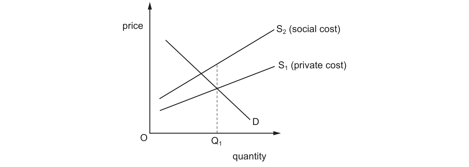
Answer: B.
The other options would each look different on the diagram. A subsidy (A) or a positive externality (C) would put the social curve BELOW the private one. A specific tax (D) shifts the private supply curve itself rather than opening a gap between two separate curves.
Cross-board concept practice · originally a CIE 9708 question, used here because the concept is the same. It is not IB Economics past-paper material.
Question 3
In the diagram, S1 is the original supply curve and D is the original demand curve. If supply shifts to S2, which area represents the change in consumer surplus?
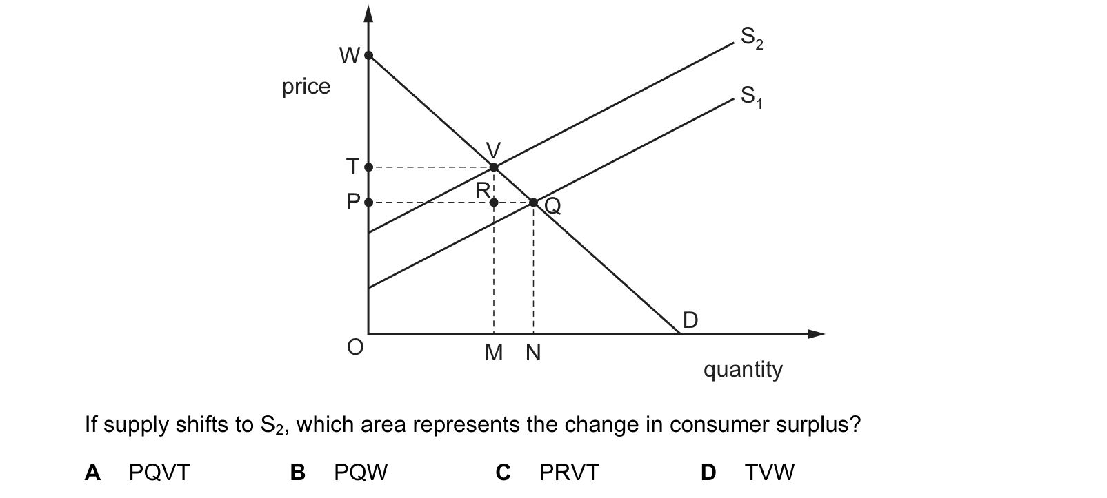
Answer: A.
Explanation:
- Consumer surplus is the area between the price that consumers are willing to pay (D curve) and the actual price (P). When supply shifts from S1 to S2, the new equilibrium price will decrease from P to P2, leading to a lower price for consumers.
- The change in consumer surplus after the shift in supply can be calculated by comparing the original consumer surplus (triangle above P and under D) and the new consumer surplus after the shift (triangle above P2 and under D).
- In the given options, area PQVT represents the change in consumer surplus after the shift in supply from S1 to S2. This area captures the decrease in consumer surplus due to the decrease in price (from P to P2) resulting from the increase in supply.
- Choice B (PQW) does not represent the change in consumer surplus accurately after the shift in supply. It only captures a portion of the original consumer surplus and does not account for the full decrease in consumer surplus due to the shift.
- Choices C (PRVT) and D (TVW) are also incorrect as they do not accurately represent the change in consumer surplus after the shift in supply.
- The correct area to represent the change in consumer surplus must consider the overall decrease in consumer surplus resulting from the decrease in price caused by the increase in supply.
What the syllabus asks for on this topicSyllabus points
Syllabus points
- Explain the law of supply and the shape of the supply curve.
- Distinguish a movement along from a shift of the supply curve.
- Explain the non-price determinants of supply.
- (HL) Use and plot a linear supply function.
Related IB Economics topics
Not the topic you were looking for? Describe what you are stuck on in your own words and we will take you to the notes that answer it.