Demand
Contents: 10 sections
The law of demand
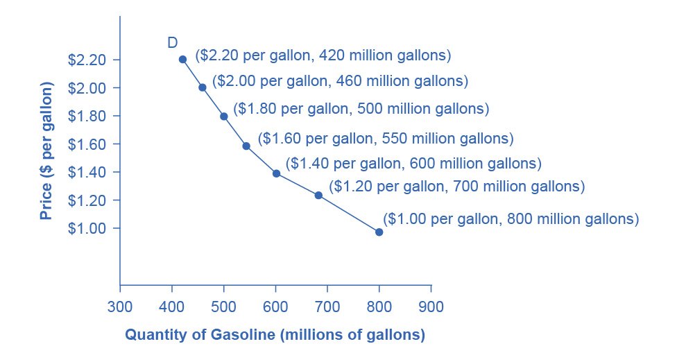
Demand is the quantity of a good consumers are willing and able to buy at each price over a given period of time.
Both halves of "willing and able" matter. Wanting a Ferrari is not demand; being able to pay for one and choosing to is. Economists call this effective demand, and it is why demand and need are different concepts, a household may urgently need medicine and register no demand for it at all if it cannot pay. That gap between need and effective demand is the seed of the equity argument in 2.12.
The law of demand states that, ceteris paribus, as price rises quantity demanded falls, and as price falls quantity demanded rises. The demand curve therefore slopes downwards.
Two effects explain the negative slope, and examiners want both named:
- Income effect: a lower price raises real purchasing power (the same money income now buys more), so consumers can afford a larger quantity.
- Substitution effect: a lower price makes the good cheaper relative to substitutes, so consumers switch towards it and away from alternatives.
(HL) The utility explanation
Demand can also be derived from diminishing marginal utility: each additional unit consumed adds less satisfaction than the one before. A rational consumer buys that extra, less-satisfying unit only if the price falls to match the lower marginal utility it delivers. Aggregating that logic across consumers gives a downward-sloping demand curve.
Note that the demand curve is therefore also a marginal benefit curve: the height of the curve at any quantity is what the marginal consumer is willing to pay, which is what that unit is worth to them. That reading is what makes consumer surplus and the welfare analysis of market failure possible later.
Key definitions
| Term | Exam-ready definition |
|---|---|
| Demand | The quantity consumers are willing and able to buy at each price. |
| Law of demand | As price rises, quantity demanded falls, ceteris paribus. |
| Movement along | A change in quantity demanded caused only by the good's own price. |
| Shift | A change in demand at every price caused by a non-price factor. |
| Ceteris paribus | "All other things equal": the assumption isolating one variable. |
| Effective demand | Demand backed by the ability and willingness to pay. |
Movement along versus a shift
This distinction earns easy marks and is the most commonly confused idea in the whole topic. The rule is simple and has no exceptions:
- A change in the good's own price causes a movement along the curve, a change in quantity demanded.
- A change in any other factor shifts the whole curve left or right, a change in demand.
The vocabulary is not decoration. Writing "a price fall increases demand" is marked wrong: a price fall increases quantity demanded. Use the two phrases precisely, because in a 10-mark answer the examiner is checking whether you understand the difference or merely have a word for it.
Non-price determinants of demand
Group them so you can retrieve them under pressure, income, related goods, tastes, market size, expectations:
- Income: for a normal good, higher income raises demand; for an inferior good, higher income lowers it, as people trade up to something better.
- Price of substitutes: a dearer substitute raises demand for this good. Tea and coffee, rail and coach.
- Price of complements: a dearer complement lowers demand for this good. Printers and ink, cars and petrol.
- Tastes and preferences: advertising, fashion, health information, social norms.
- Number of consumers: population growth, or access to a new market.
- Future expectations: expecting prices to rise later raises demand now.
- Interest rates and credit: for goods usually bought on credit (cars, housing), cheaper borrowing raises demand.
A note on "inferior". An inferior good is defined purely by its negative income effect, not by quality. Bus travel, own-brand food and instant noodles are the standard examples: nothing is wrong with them, but people buy less of them as they get richer. Calling any cheap good inferior is a frequent error, and the test is always what happens to demand when income rises.
(HL) The linear demand function
Paper 3 expresses demand algebraically:
Qd = a − bP
where a is the quantity demanded if the good were free, and b measures how strongly quantity responds to price, the steeper the response, the larger b.
Worked example. Qd = 200 − 5P.
| Price | Quantity demanded |
|---|---|
| \$0 | 200 |
| \$10 | 150 |
| \$20 | 100 |
| \$30 | 50 |
| \$40 | 0 |
To plot it, find the two intercepts: quantity is 200 when P = 0, and quantity is zero when 200 − 5P = 0, so P = 40. Join them.
What changes what. A change in a shifts the whole curve; that is a non-price determinant at work. A change in b rotates it, altering how responsive quantity is to price. A change in P alone moves you along the curve. Being able to say which parameter a described event changes is exactly the movement-versus-shift distinction in algebraic form.
Individual and market demand
Market demand is the horizontal sum of all individual demand curves: at each price, add up the quantities every consumer would buy. This is why an increase in the number of consumers shifts market demand right without any individual changing their behaviour at all.
Worked example
The price of petrol rises sharply. What happens in the market for large cars?
- Petrol and large cars are complements; they are consumed together
- running a large car becomes more expensive overall
- at every price, fewer consumers are willing and able to buy one
- the demand curve for large cars shifts left, from D₁ to D₂.
This is a shift, because the price of petrol is a non-price factor from the perspective of the car market. It is not a movement along the car demand curve, the price of cars has not changed.
Follow it through to the market outcome: with supply unchanged, the leftward demand shift produces a lower equilibrium price and a lower quantity traded for large cars.
Two things to add for the higher marks. How far price falls rather than quantity depends on the elasticity of supply, where supply is inelastic in the short run, most of the adjustment lands on price. And there is a second market to mention: demand for small, fuel-efficient cars shifts right, because they are substitutes. Tracing the effect into the related market shows the interdependence the syllabus cares about.
Common exam mistakes
- Calling a shift a "movement", or vice versa.
- Writing that a price change "increases demand", it changes quantity demanded.
- Forgetting to state ceteris paribus when explaining the law of demand.
- Explaining the downward slope with only one of the income and substitution effects.
- Confusing an inferior good (negative income effect) with a cheap or low-quality good.
- Shifting demand for a good when its own price changed.
- (HL) Reading a as a price or b as an elasticity; they are the intercept and the slope parameter.
Exam technique
Label diagrams fully: axes as price and quantity, curves as D₁ and D₂, and both the original and new equilibrium marked with dotted lines to each axis.
State the cause of a shift explicitly, then trace the consequence: cause → shift → new equilibrium price and quantity. "Demand shifts right" is a description; "demand shifts right because incomes rose and this is a normal good, so equilibrium price and quantity both rise" is analysis.
When given a demand function, find both intercepts before drawing anything. Two points fix a straight line, and the intercepts are the two easiest to compute.
For evaluation, useful angles are the size of the shift, the elasticity of supply (which determines how much of the adjustment falls on price rather than quantity), and the time frame.
Quick revision
- Demand = willing and able to buy; the curve slopes down via the income and substitution effects.
- (HL) Diminishing marginal utility gives the same result; the demand curve is a marginal benefit curve.
- Own price → movement along (quantity demanded). Anything else → shift (demand).
- Determinants: income, substitutes, complements, tastes, number of buyers, expectations, credit.
- Inferior is defined by a negative income effect, not by low quality.
- Market demand is the horizontal sum of individual demands.
- Substitutes move demand the same way as their price; complements the opposite way.
- (HL) Qd = a − bP; a shifts the curve, b rotates it, P moves you along it.
Check you have it
Cross-board concept practice · originally a CIE 9708 question, used here because the concept is the same. It is not IB Economics past-paper material.
Question 1
The diagrams show initial equilibrium positions at Y1P1. Which diagram reflects the impact on an economy of higher unit wage costs and an improvement in the balance of trade?
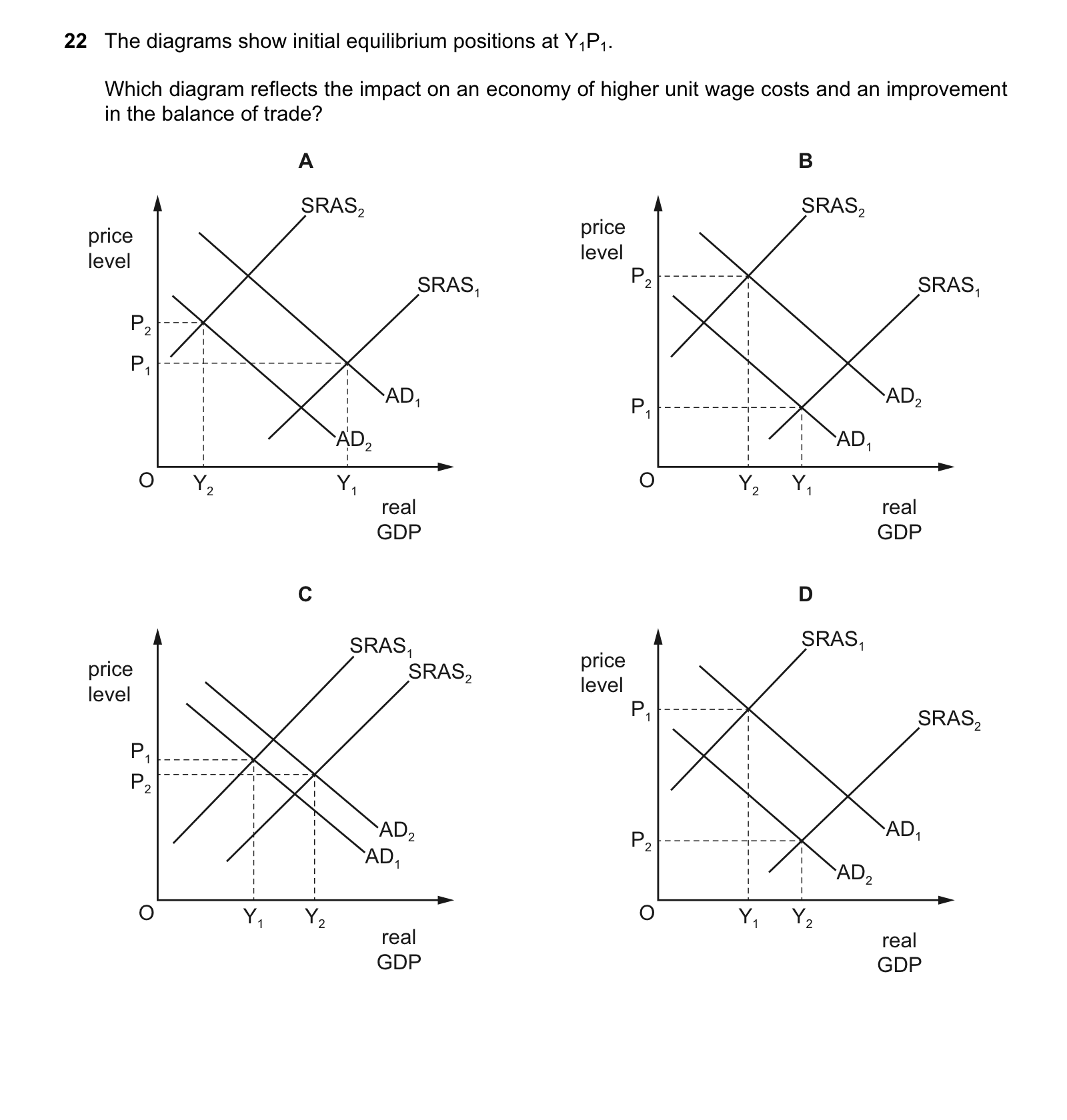
Answer: B.
Explanation:
- An improvement in the balance of trade means that the country is exporting more than it is importing, leading to an increase in net exports and ultimately boosting the aggregate demand (AD) curve.
- Higher unit wage costs would lead to an increase in production costs for firms, shifting the short-run aggregate supply (SRAS) curve to the left as they would need to increase prices to maintain profit margins.
- The combination of an upward shift in the AD curve and a leftward shift in the SRAS curve would lead to an increase in the price level (from P1 to P2) and a decrease in real GDP (from Y1 to Y2), which is depicted in diagram B.
Cross-board concept practice · originally a CIE 9708 question, used here because the concept is the same. It is not IB Economics past-paper material.
Question 2
The diagram shows an industry’s demand and supply curves. The industry increases supply from S1 to S2. Which area shows the total gain in society’s economic welfare?
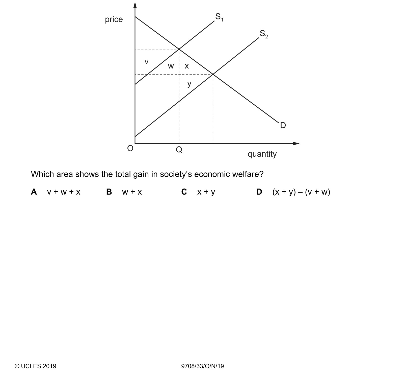
Answer: C.
Cross-board concept practice · originally a CIE 9708 question, used here because the concept is the same. It is not IB Economics past-paper material.
Question 3
The diagram shows the short-run equilibrium for a firm operating in a monopolistically competitive market. What is not likely to occur at the long-run equilibrium?
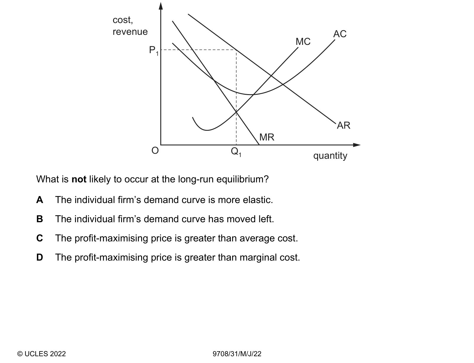
Answer: C.
What the syllabus asks for on this topicSyllabus points
Syllabus points
- Explain the law of demand and the shape of the demand curve.
- Distinguish a movement along from a shift of the demand curve.
- Explain the non-price determinants of demand.
- (HL) Explain demand using the assumptions of utility.
- (HL) Use and plot a linear demand function.
Related IB Economics topics
Not the topic you were looking for? Describe what you are stuck on in your own words and we will take you to the notes that answer it.