Policies to Correct Market Failure

1. Why this topic matters

At AS Level you learned that markets can fail. Topic 8.1 asks the harder question: given that a market has failed, what should a government actually do about it, and will the intervention improve matters?

This topic is where a large share of Paper 4 marks are won and lost, because it rewards two things at once:

• precise analysis of how a named policy changes incentives, prices and quantities; and
• honest evaluation of whether that policy achieves allocative efficiency in practice.

The single most common weakness is describing a policy rather than analysing it. "The government could impose a tax" earns very little. Explaining that a tax equal to the marginal external cost at the socially optimal output internalises the externality, shifts the supply curve from S to S plus tax, and moves output from Q1 to Q\*, earns a great deal.

Keep three ideas separate throughout:

• allocative efficiency occurs where price equals marginal cost, or where marginal social benefit equals marginal social cost;
• productive efficiency occurs where a firm produces at minimum average cost; and
• equity is about fairness of distribution and is a separate objective, covered in 8.2.

A policy can improve one and worsen another. Saying so is evaluation.

2. The efficiency target

2.1 The social optimum

The socially optimum output occurs where marginal social benefit (MSB) equals marginal social cost (MSC).

• MSB is the sum of marginal private benefit (MPB) and marginal external benefit (MEB).
• MSC is the sum of marginal private cost (MPC) and marginal external cost (MEC).

A free market equilibrium occurs where MPB equals MPC. Where external costs or benefits exist, that private equilibrium differs from the social optimum, and the gap generates a welfare loss (also called deadweight loss).

2.2 The direction of the failure

Getting the direction right is essential before choosing a policy.

• Negative externality in production: MSC lies above MPC. The market over-produces. Output must fall.

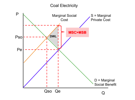
• Negative externality in consumption: MSB lies below MPB. The market over-consumes. Consumption must fall.
• Positive externality in production: MSC lies below MPC. The market under-produces. Output must rise.
• Positive externality in consumption: MSB lies above MPB. The market under-consumes. Consumption must rise.

A policy that reduces output when the failure is under-provision will lose marks however well it is described.

2.3 The size of the correction

The theoretically correct correction equals the value of the external cost or benefit at the socially optimal output, not at the free market output. This is a subtle point that strong candidates make explicitly, because MEC often varies with output.

3. Indirect taxation

3.1 The mechanism

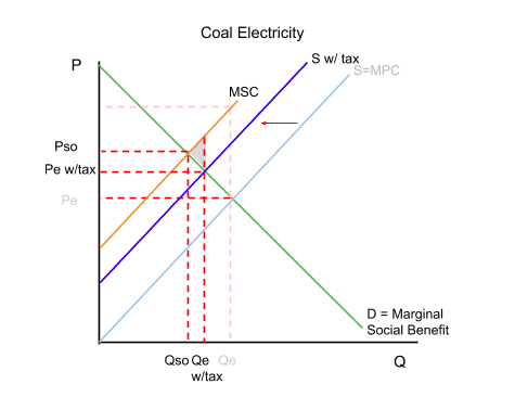
An indirect tax raises a producer's costs, shifting the supply curve upward and to the left. Where the tax per unit equals the marginal external cost at the optimum, private cost is brought into line with social cost. The externality is then fully internalised.

Output falls from the free market quantity towards the social optimum and the price to consumers rises. Whether the welfare loss is reduced or eliminated depends entirely on the size of the tax, and the diagram below is drawn for the more realistic case in which the tax is smaller than the external cost: output stops at Qe with tax, short of Qso, and a small triangle of welfare loss survives.

3.2 When the tax is smaller than the external cost

Setting the tax exactly equal to the marginal external cost is the textbook case, not the usual one. Governments rarely know the external cost precisely, and a tax large enough to close the gap is often politically unattractive, so in practice the tax is frequently less than the external cost.

The consequence is worth being able to draw. Supply shifts up by less than the full vertical gap between private and social cost, so output falls only part of the way from the free market quantity to the social optimum. The welfare loss shrinks. It does not disappear.

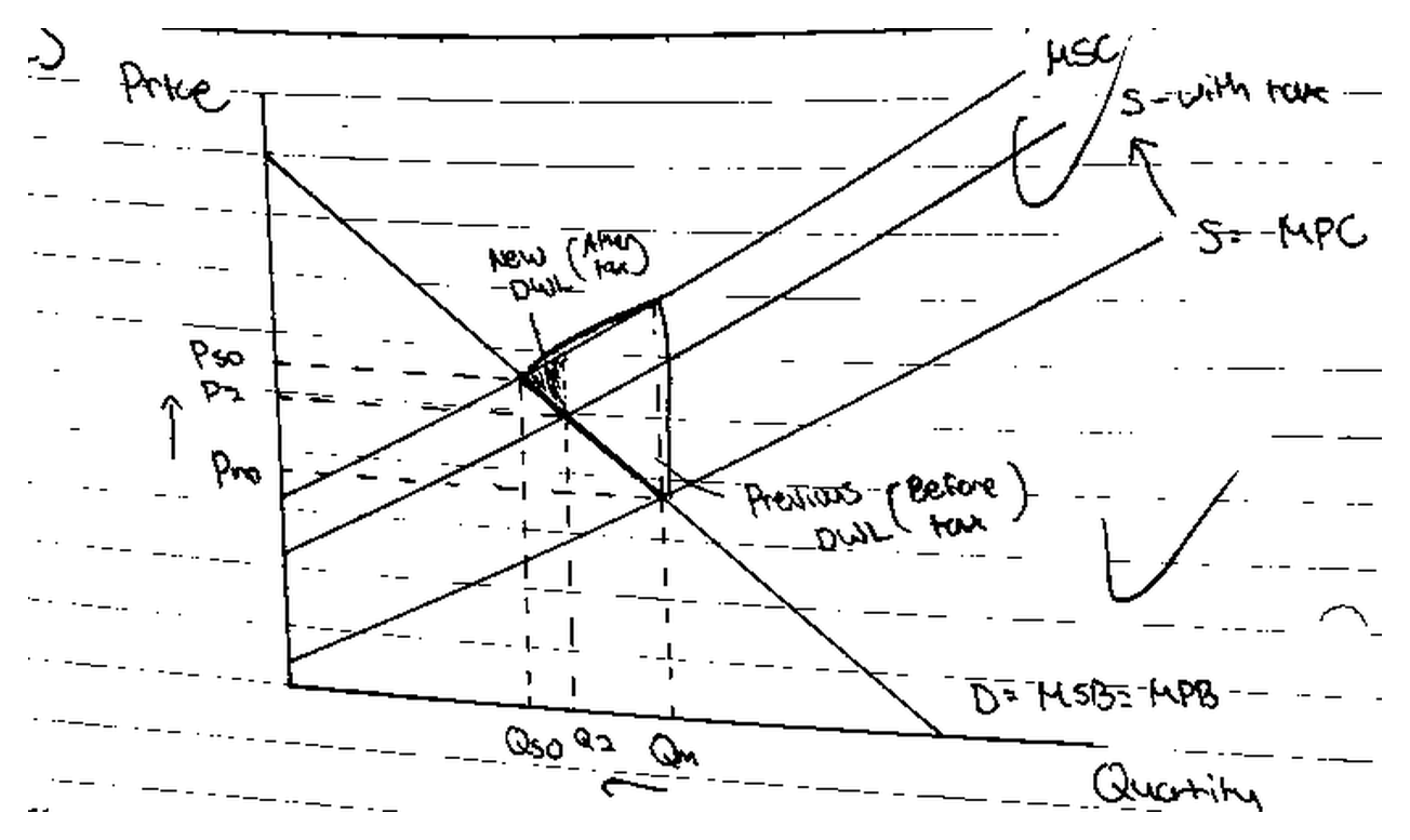
This version labels both triangles, which the diagram above does not: the large one is the loss before the tax, the smaller one inside it is what is left after. Seeing the two together is what makes the point concrete, because the tax is doing real work and still leaving a loss behind.

So an answer that says a tax "corrects" or "removes" the externality is claiming the special case where the tax equals the marginal external cost at the optimum. Saying which case you are in, and why, is an evaluation mark rather than a knowledge one.

3.3 Specific and ad valorem taxes

• A specific tax is a fixed amount per unit. It shifts supply upward by a constant vertical distance and the curves stay parallel.
• An ad valorem tax is a percentage of price. The vertical shift widens as price rises, so the new supply curve pivots away from the original.

3.4 Incidence and elasticity

The burden of the tax is shared between consumers and producers according to relative elasticities.

• The more inelastic demand is relative to supply, the greater the share borne by consumers.
• The more elastic demand is relative to supply, the greater the share borne by producers.

This matters for evaluation. Where demand is highly inelastic, as with addictive goods, a tax raises substantial revenue but reduces quantity only slightly, so the efficiency objective is poorly served even though the revenue objective is met.

3.5 Worked calculation

Suppose the free market equilibrium for a chemical is 900 tonnes, and each tonne generates an external cost of $40. A specific tax of $40 per tonne is imposed.

• Supply shifts vertically upward by $40 at every quantity.
• Suppose the new equilibrium quantity is 750 tonnes and the new consumer price is $128, against a pre-tax price of $104.
• Consumer burden per unit: $128 minus $104 equals $24.
• Producer burden per unit: $40 minus $24 equals $16.
• Total tax revenue: $40 multiplied by 750 equals $30,000.
• Consumers bear 24/40, which is 60 per cent of the burden.

The reduction in output of 150 tonnes is the efficiency gain. The revenue is a separate consequence, not a measure of success.

3.6 Evaluation

Strengths:

• works through the price mechanism rather than replacing it;
• raises revenue that can fund related spending; and
• leaves firms free to choose how to reduce output or emissions, so abatement occurs where it is cheapest.

Weaknesses:

• the external cost must be valued in money, which is difficult and contested;
• inelastic demand limits the quantity effect;
• the tax is regressive where the good forms a larger share of low income budgets; and
• production may relocate to jurisdictions without the tax, so global external costs are unchanged.

4. Subsidies

4.1 The mechanism

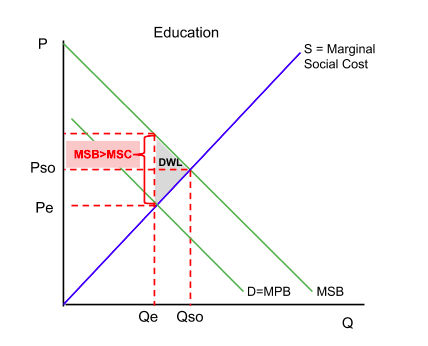
A subsidy lowers a producer's costs, shifting supply downward and to the right, or it can be paid to consumers to shift demand rightward. Where a positive externality causes under-consumption, a subsidy equal to the marginal external benefit at the optimum moves output up towards the social optimum.

Price to consumers falls, quantity rises, and the welfare loss from under-provision is reduced.

4.2 Worked calculation

A government subsidises vaccinations at $18 per dose.

• Quantity rises from 40,000 to 55,000 doses.
• Consumer price falls from $30 to $19.
• Government spending: $18 multiplied by 55,000 equals $990,000.
• Consumer gain per dose: $30 minus $19 equals $11, so consumers capture 11/18 of the subsidy.
• Producer gain per dose: $18 minus $11 equals $7.

4.3 Evaluation

Strengths:

• directly raises consumption of merit goods;
• can be targeted at particular groups or regions; and
• may generate long term benefits that exceed the immediate cost.

Weaknesses:

• opportunity cost of the government spending;
• risk of producer inefficiency where the subsidy is guaranteed;
• the true value of the external benefit is hard to estimate; and
• much of the benefit may accrue to those who would have consumed anyway.

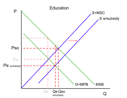
Read this against the tax in 3.2 and the pattern is the same in mirror image. The subsidised quantity stops short of Qso, because the subsidy drawn here is smaller than the marginal external benefit. Under-consumption is reduced, not abolished, and the same evaluation applies: whether a subsidy corrects a positive externality or merely narrows it depends entirely on its size against an external benefit the government has to estimate.

5. Regulation and legislation

▶

5.1 The mechanism

Regulation sets rules directly rather than adjusting prices. Examples include emissions limits, minimum school leaving ages, bans on particular substances, licensing requirements and compulsory safety standards.

Regulation is a command approach: it specifies the outcome rather than changing incentives.

5.2 Evaluation

Strengths:

• provides certainty about the quantity outcome, which taxes do not;
• appropriate where any level of the activity is unacceptable, for example toxic waste; and
• simple for the public to understand.

Weaknesses:

• requires monitoring and enforcement, both costly;
• a uniform standard is inefficient because abatement costs differ across firms, so the same reduction could be achieved more cheaply by allowing trade;
• provides no incentive to reduce beyond the limit; and
• may create black markets where a ban removes legal supply.

6. Tradable pollution permits

▶

6.1 The mechanism

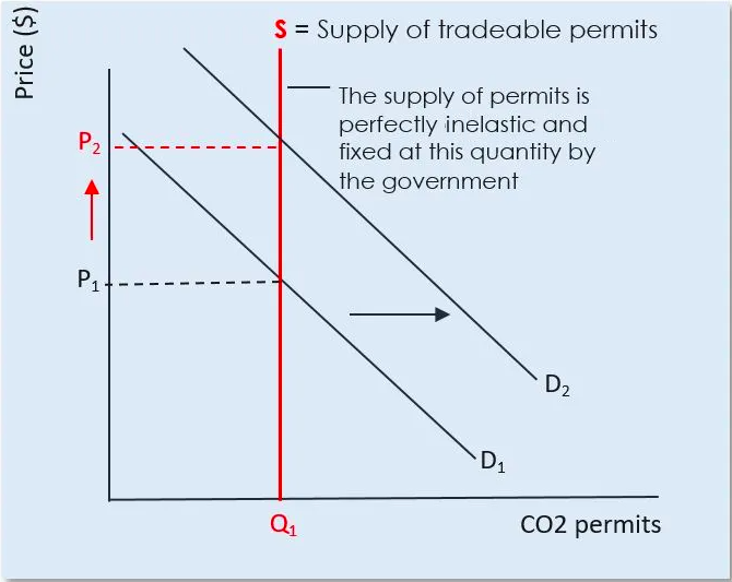
The authority sets a total quantity of permitted emissions and issues permits equal to that total, either free or by auction. Firms may then buy and sell permits.

A firm with low abatement costs reduces emissions and sells its surplus permits. A firm with high abatement costs buys permits instead of abating. Total emissions are fixed by the cap, but the reduction happens where it costs least.

6.2 Why this is efficient

The permit price settles at the marginal abatement cost of the marginal firm. Every firm with abatement costs below the permit price abates; every firm above it buys. Total abatement cost is therefore minimised for the given cap.

6.3 Worked example

Two firms each emit 100 tonnes. The cap is 120 tonnes in total, so 60 permits each are issued.

• Firm A's abatement cost is $30 per tonne; Firm B's is $70 per tonne.
• Without trade, each abates 40 tonnes: total cost equals 40 multiplied by $30 plus 40 multiplied by $70, which is $1,200 plus $2,800, equal to $4,000.
• With trade at a permit price of $50, Firm A abates all 80 tonnes for $2,400 and sells 40 permits to Firm B for $2,000.
• Firm A's net cost: $2,400 minus $2,000 equals $400. Firm B's cost: $2,000.
• Total cost: $2,400, against $4,000 without trade. The same environmental outcome is achieved for $1,600 less.

6.4 Evaluation

Strengths:

• the environmental outcome is certain because the cap is fixed;
• abatement occurs at least cost; and
• the cap can be tightened over time.

Weaknesses:

• setting the initial cap requires the same valuation problem as a tax;
• permits issued free confer windfall gains on existing polluters;
• monitoring emissions accurately is expensive; and
• the scheme covers only the firms inside it, so activity may shift outside.

7. State provision

7.1 The mechanism

Where a good is a public good, the free rider problem means the market provides little or none of it, because non-excludability removes the ability to charge. Direct state provision funded through taxation is then the standard response.

State provision is also used for merit goods where the external benefit is large and access is judged a matter of equity, for example basic healthcare and education.

7.2 Evaluation

Strengths:

• overcomes non-excludability, which no price based policy can;
• can guarantee universal access; and
• avoids the under-consumption associated with merit goods.

Weaknesses:

• no price signal means quantity and quality decisions rest on administrative judgement;
• funding has an opportunity cost and may require distortionary taxation;
• absence of competition can weaken the incentive to control costs; and
• excess demand may appear as queues or rationing rather than higher prices.

8. Information provision

8.1 The mechanism

Where the failure arises from information failure rather than externality, correcting the information may be the appropriate remedy. Examples include compulsory nutritional labelling, health warnings, fuel efficiency ratings and published school performance data.

If consumers systematically underestimate a private cost, their MPB curve lies above their true benefit. Better information shifts perceived MPB towards the true curve and reduces consumption without any tax.

8.2 Evaluation

Strengths:

• preserves consumer choice, which taxes and bans restrict;
• addresses the actual cause where the problem is ignorance; and
• relatively low cost.

Weaknesses:

• information may be ignored, misunderstood or outweighed by addiction;
• effects are slow and hard to measure; and
• does nothing where the problem is an external cost rather than misinformation.

9. Property rights

9.1 The mechanism

Many external costs arise because no one owns the resource being damaged. Where property rights over a resource are absent, no one has the incentive or standing to prevent its degradation. This is the tragedy of the commons.

Assigning and enforcing property rights allows the owner to charge for use or to seek compensation for damage, so the external cost becomes a private cost.

9.2 Evaluation

Strengths:

• addresses the underlying cause rather than the symptom;
• allows private bargaining without continuing state involvement; and
• avoids the valuation problem, since the parties negotiate.

Weaknesses:

• impossible for genuinely global resources such as the atmosphere;
• bargaining fails where many parties are involved, because transaction costs are high; and
• the outcome depends on who receives the rights, which is a question of equity.

10. Behavioural policies

Governments increasingly use nudges, which change the framing or default of a choice without removing options. Examples include automatic enrolment in pension schemes, placing healthier food at eye level, and default organ donation registration.

Evaluation: nudges are cheap and preserve choice, but their effects are often small, may fade, and can be reversed by commercial nudges pushing the other way. They are best treated as a complement to, not a substitute for, price based policy.

11. Choosing between policies

A strong Paper 4 answer compares rather than lists. The choice depends on:

• the source of the failure: information failure calls for information; missing markets call for property rights or state provision; externalities call for taxes, subsidies or permits;
• elasticity: price based policies work poorly where demand is very inelastic;
• whether quantity certainty matters: permits and regulation fix quantity, taxes fix price;
• administrative capacity: permits and cost-benefit analysis demand data and enforcement that some governments lack;
• distributional effects: taxes on necessities are regressive; and
• the risk of government failure, covered in 8.4.

<!-- merged from the former 8.4; syllabus 8.1.2 is government failure in microeconomic intervention -->

12. The counterfactual

The correct test is always: what would have happened otherwise?

Suppose a government subsidises public transport and congestion still rises. That is not evidence of failure by itself. Congestion might have risen further without the subsidy, in which case the policy succeeded despite the headline. Establishing the counterfactual is difficult, which is one reason government failure is hard to prove and easy to assert.

Strong answers make this explicit: "this appears to be government failure, but only if congestion would have been lower in the absence of the subsidy, which the data does not show."

13. Causes of government failure

16.1 Imperfect information

To set a corrective tax at the right level, a government must know the marginal external cost at the socially optimal output. That requires valuing things which have no market price: a life shortened by air pollution, an hour lost in traffic, the loss of a habitat.

Consequences:

• A tax set below the true external cost leaves the market over-producing, so the welfare loss shrinks but does not disappear.
• A tax set above it pushes output below the social optimum, creating a new welfare loss on the other side. This is government failure in the strict sense, because the allocation is now wrong in the opposite direction.

The same problem applies to subsidies, to setting a cap for tradable permits, and to cost-benefit analysis in 8.5.

16.2 Administrative and enforcement costs

Intervention consumes real resources: collecting a tax, inspecting emissions, administering means tests, running a licensing regime, prosecuting breaches.

Where these costs exceed the welfare gain from the correction, the intervention makes society worse off even though it works as designed. This is why very small externalities are often left uncorrected: the administrative cost of correcting them would exceed the harm.

16.3 Unintended consequences

Interventions change incentives, and people respond in ways the designer did not anticipate.

• A maximum price below equilibrium creates excess demand, and the shortage may be resolved by queues, rationing or a black market in which the price exceeds the free market price and quality is unregulated.
• A minimum price creates excess supply, which the authority may have to buy and store at cost, as in agricultural buffer stocks.
• A tax on a demerit good with inelastic demand raises revenue but barely changes consumption, while imposing a regressive burden.
• Subsidising an input may encourage its wasteful use, as with water or fertiliser subsidies leading to over-extraction and run-off.
• Landfill taxes raise the cost of legal disposal and can increase illegal dumping.

Naming the mechanism, not just the outcome, is what earns the marks.

16.4 Distortion of price signals

Prices carry information about relative scarcity and coordinate millions of decentralised decisions. Interventions that fix or distort prices suppress that information.

Under a maximum price, producers receive a signal that the good is less scarce than it is, so they supply less exactly when more is needed. Under a permanent subsidy, high cost producers survive who would otherwise have exited, so resources stay in a low value use. This is a productive efficiency loss as well as an allocative one.

16.5 Regulatory capture

Regulatory capture occurs where the regulator comes to act in the interests of the industry it regulates rather than the public.

The mechanism is informational and structural. The regulator depends on the firms for data; the industry has concentrated, well funded interests while consumers are dispersed and each has little at stake; and staff move between regulator and industry. The result may be weak price caps, lenient standards or barriers that protect incumbents.

16.6 Political self-interest and the electoral cycle

Governments face re-election, so decisions may be shaped by what is visible before the next election rather than by long run welfare. Policies with concentrated, visible benefits and dispersed, delayed costs are politically attractive even when the net effect is negative. Long payback investments, and taxes whose benefits accrue to the next generation, are systematically under-supplied.

16.7 Conflicting objectives

A government pursues several objectives at once, and microeconomic interventions frequently trade against one another.

• A carbon tax improves allocative efficiency and is regressive, so it conflicts with equity.
• A minimum wage raises low pay and may reduce employment, so equity conflicts with efficiency.
• Protecting an industry preserves jobs in the short run and reduces the incentive to become competitive.

Where objectives conflict, any choice sacrifices something, and calling the sacrificed objective a "failure" is usually wrong. It is a trade-off.

16.8 Time lags

Intervention involves recognition, decision, implementation and effect lags. By the time a policy takes effect, the conditions that justified it may have changed, so the policy is destabilising rather than corrective. Agricultural support and housing supply policy are common examples.

16.9 Moral hazard

Where intervention insures people against the consequences of their decisions, behaviour changes. Guaranteed rescue may encourage excessive risk taking; guaranteed prices may encourage production regardless of demand. The insurance itself alters the incentives that made it necessary.

14. Worked example: a maximum price

A government imposes a maximum rent of $600 per month where the equilibrium is $900.

Analysis:

• Quantity demanded rises, because rent is lower.
• Quantity supplied falls, because letting is less profitable, and in the long run some landlords convert or sell property.
• Excess demand appears, so accommodation is rationed by waiting lists, by landlord discretion or by informal side payments.
• Maintenance falls, because at a controlled rent landlords face excess demand regardless of quality.

Intended effect: tenants pay less. Actual effect: those who hold a controlled tenancy pay less, while those seeking one may be unable to rent at all, and the quality of the stock declines.

Whether this is government failure depends on the comparison. If the welfare gain to existing tenants exceeds the loss to excluded households and the deterioration in quality, the policy is a costly success. If it does not; it is government failure. State the condition rather than assuming the answer.

15. Worked example: an agricultural buffer stock

A buffer stock scheme aims to stabilise the price of a commodity around a target by buying when the price would otherwise fall and selling when it would otherwise rise. It is the classic CIE case because it can fail in several ways at once.

16.1 How it is meant to work

The authority sets a target price band with a floor and a ceiling.

• In a good harvest, supply shifts right and the price would fall below the floor, so the authority buys the surplus and stores it. Demand is effectively increased, holding the price at the floor.
• In a poor harvest, supply shifts left and the price would rise above the ceiling, so the authority sells from the store. Supply is effectively increased, holding the price at the ceiling.

If the target price is set at the long run average, purchases in good years are financed by sales in bad years, and the scheme is self-funding.

16.2 Where it fails

• The target price is set too high, usually for political reasons, because farmers are an organised interest and consumers are dispersed. Purchases then exceed sales year after year, stocks grow without limit and the scheme runs a permanent deficit.
• Storage costs are real and recurring, and perishable commodities deteriorate, so a large stock is an ongoing drain even before any price effect.
• A guaranteed floor encourages over-production, because it removes downside risk. Supply shifts right permanently, which makes the surplus structural rather than cyclical.
• Resources are locked into a low value use, since land and labour stay in a crop the market does not want at that price.
• Disposal distorts other markets, since dumping the surplus abroad depresses world prices and can damage producers in developing countries.

16.3 Worked numbers

Suppose the floor is $220 per tonne, and at that price supply is 900,000 tonnes and demand is 760,000 tonnes.

• Surplus purchased: 140,000 tonnes.
• Cost of purchase: 140,000 multiplied by $220 equals $30.8 million.
• Storage at $12 per tonne per year adds $1.68 million a year, and rises as the stock accumulates.

If the following year is also good, the authority buys again while still holding the first surplus. The scheme now owns 280,000 tonnes, has spent over $61 million, and faces storage costs of $3.36 million a year on a stock it may never be able to sell without depressing the very price it is defending.

This is government failure in the strict sense: the intervention has created a misallocation, an ongoing fiscal cost and an incentive distortion, and the price instability it addressed was a smaller problem than the permanent surplus it produced.

The evaluation, as always, is conditional. A buffer stock set at the genuine long run average price, with credible storage capacity and enforcement against over-production, can reduce harmful volatility for farmers whose incomes are otherwise unpredictable. The failure lies in the setting of the price, not in the idea.

16. Reducing the risk of government failure

Examiners reward candidates who move past listing causes to suggesting mitigations.

• Use market based instruments where possible, since taxes and tradable permits leave the price mechanism working and let firms find the cheapest response.
• Pilot and evaluate before national rollout, and build in review dates.
• Use independent agencies with statutory objectives, to insulate technical decisions from the electoral cycle.
• Improve information through better data collection and by requiring firms to disclose, which reduces the valuation problem and the capture problem together.
• Design for the response, anticipating how the taxed or regulated party will adapt.
• Compare against the counterfactual explicitly when evaluating.
• Sunset clauses, so a policy lapses unless actively renewed.

<!-- merged from the former 8.6; syllabus 8.1.1 lists nationalisation and privatisation as measures under 8.1 -->

17. Nationalisation

20.1 Definition

Nationalisation is the transfer of an industry or firm from private to public ownership, so that it is owned and controlled by the state.

20.2 The case for

• Natural monopoly. Where economies of scale are so large that one firm can supply the whole market at lower average cost than several, competition is wasteful because it duplicates infrastructure. Water networks, rail track and electricity transmission are standard examples. Public ownership avoids a private monopoly exploiting that position.
• Externalities. A state owner can take social costs and benefits into account rather than maximising profit, for example maintaining a rural rail service whose social benefit exceeds its revenue.
• Equity and universal service. The state can require supply to remote or poor households at a uniform price, which a profit maximiser would not serve.
• Strategic importance. Energy, defence and water may be judged too important to leave to private decision, particularly where security of supply matters.
• Macroeconomic control. Public ownership gives a government a direct instrument for employment and investment.

20.3 The case against

• X-inefficiency. Without the discipline of competition or the threat of bankruptcy, average costs drift above the minimum attainable. Managers face weak incentives to control cost.
• Absence of the profit motive removes the clearest signal of whether resources are being used well.
• Political interference. Investment and pricing decisions may follow the electoral cycle rather than long run efficiency, which is the government failure of 8.4 applied to ownership.
• Opportunity cost of public funds and the burden of subsidising loss making operations.
• Diseconomies of scale in very large state organisations, through coordination and communication problems.

18. Privatisation

20.1 Definition and forms

Privatisation is the transfer of ownership from the public to the private sector. It takes several forms:

• outright sale of assets, usually by share issue;
• contracting out, where the state still funds a service but a private firm delivers it;
• deregulation, removing legal barriers to entry so private firms may compete; and
• public private partnerships, where private capital finances public infrastructure in return for a stream of payments.

20.2 The case for

• Productive efficiency. The profit motive and the threat of takeover or bankruptcy give a private owner strong incentives to cut costs, so average costs should fall towards the minimum.
• Allocative efficiency, where privatisation is combined with genuine competition, since firms must respond to consumer preferences to survive.
• Dynamic efficiency. Access to private capital markets and the prospect of profit may raise investment and innovation.
• Revenue from the sale, and removal of ongoing subsidies from the budget.
• Removal of political interference from operational decisions.

20.3 The case against

• A private monopoly may replace a public one. Where the industry is a natural monopoly, ownership changes but market power does not, so price may rise towards the profit maximising level and output fall below the allocatively efficient level.
• Loss of social objectives. A profit maximiser withdraws from unprofitable routes, regions or customers, damaging equity and universal service.
• Cherry picking. New entrants may take only the profitable segments, leaving the incumbent with the loss making obligations, which raises the cost of universal provision.
• Short termism, where pressure for dividends reduces long term investment in infrastructure.
• Job losses during cost cutting, with regional concentration.
• Assets may be sold below their true value, transferring wealth from taxpayers to shareholders.

20.4 The decisive question

Whether privatisation improves welfare depends far less on ownership than on market structure after the sale. Where the market is genuinely contestable, competition disciplines the firm and the efficiency gains are real. Where it remains a natural monopoly, everything depends on the quality of regulation.

That sentence is the spine of any good essay on this topic.

19. Regulating a privatised monopoly

20.1 Price cap regulation

The regulator limits the rate at which the firm may raise prices, commonly expressed as RPI minus X, where RPI is the inflation rate and X is an efficiency factor.

If inflation is 4 per cent and X is set at 3, the firm may raise prices by 1 per cent. Since its costs rise with inflation; it can only maintain or improve its profit margin by cutting costs faster than the cap, so the scheme creates an incentive for productive efficiency and passes some of the gain to consumers.

Worked illustration. A water company has average cost of $200 per household and charges $260. Inflation is 4 per cent, X is 3.

• Permitted price next year: $260 multiplied by 1.01, which is $262.60.
• If costs rise with inflation to $208, the margin narrows from $60 to $54.60.
• If instead the firm cuts real costs by 2 per cent, costs are approximately $203.84 and the margin is $58.76.

Evaluation: setting X requires the regulator to know the firm's scope for cost reduction, and the firm has every incentive to overstate its costs. Too high an X threatens investment and service quality; too low an X leaves consumers paying monopoly prices. This is the information asymmetry of 8.4 in a specific form.

20.2 Rate of return regulation

The regulator caps the profit the firm may earn on its capital. This protects consumers from excessive profit but creates a perverse incentive: because permitted profit rises with the capital base, the firm may over-invest in capital it does not need, which is inefficient.

20.3 Quality and service standards

Because a firm under a price cap can cut costs by cutting quality, price regulation is normally accompanied by minimum standards for reliability, safety and service, with penalties for breach.

20.4 Yardstick competition

Where several regional monopolies exist, the regulator can compare their costs and set each one's allowance by reference to the others' performance. This recreates some of the discipline of competition without requiring firms to compete for the same customers.

20. Competition policy

Competition policy is the set of rules constraining firm behaviour to protect consumers and efficiency, applied regardless of ownership.

20.1 Merger control

Mergers above a threshold may be investigated and blocked, or permitted with conditions such as selling part of the business. The test is whether the merger substantially reduces competition.

Evaluation: mergers can also raise efficiency through economies of scale, so blocking one has a cost. The authority must weigh the loss of competition against the gain in scale, which is a genuine judgement rather than a rule.

20.2 Prohibition of anti-competitive agreements

Cartels, where firms agree to fix prices, restrict output or share markets, are prohibited because they replicate monopoly outcomes without monopoly's efficiency justification.

Detection is difficult because agreements are secret, so authorities use leniency programmes that grant immunity to the first member to confess. This exploits the instability of collusion: each member gains from defecting first, which is a prisoner's dilemma.

20.3 Control of abuse of a dominant position

A firm with substantial market power may be prohibited from predatory pricing, from refusing access to essential infrastructure, or from tying products together to extend its power into another market. Dominance itself is not unlawful; abusing it is.

20.4 Promoting contestability

Since a market's behaviour depends on the threat of entry as well as the number of incumbents, policy may focus on lowering barriers to entry: removing legal restrictions, requiring incumbents to grant access to networks, and reducing sunk costs. A perfectly contestable market can produce competitive outcomes even with one firm, because the threat of hit and run entry disciplines pricing.

21. Integrated analysis and common traps

12.1 A complete chain

For a negative production externality: MSC exceeds MPC, so the free market produces Q1 where MPB equals MPC, above the optimum Q\ where MSB equals MSC. A specific tax equal to MEC at Q\ shifts supply from S to S plus tax, raising price and cutting output to Q\. The welfare loss triangle between Q\ and Q1 is eliminated. Evaluation then asks whether MEC was valued correctly and whether demand is elastic enough for the output effect to be meaningful.

12.2 Common examination errors

• Treating tax revenue as the measure of success rather than the change in quantity.
• Applying a tax to a positive externality, or a subsidy to a negative one.
• Setting the correction equal to the externality at the free market output rather than at the optimum.
• Asserting that a policy "will solve" the failure with no conditions attached.
• Confusing efficiency arguments with equity arguments.
• Describing a diagram without stating what happens to price, quantity and welfare loss.

22. Paper 3 and Paper 4 mastery

For Paper 3 multiple choice, the recurring tests are: identifying the direction of the failure, reading the effect of a tax or subsidy on a diagram, and calculating tax incidence from elasticities.

For Paper 4 essays, structure an evaluation around conditions rather than opinions. "A tax is effective provided that the external cost can be valued, demand is sufficiently elastic, and production does not relocate" is worth more than "a tax may not work".

Always finish an evaluation with a judgement that follows from the analysis, and state the condition on which it depends.

23. Final checklist

A fully prepared learner can:

• identify the direction and cause of a market failure from a description or diagram;
• state the social optimum condition and locate it on a diagram;
• explain how an indirect tax internalises a negative externality;
• calculate tax incidence and revenue from given prices and quantities;
• explain how a subsidy corrects under-consumption and calculate its cost;
• compare regulation with price based policy on cost and certainty grounds;
• explain why tradable permits minimise total abatement cost, with a numerical example;
• justify state provision from non-excludability rather than from fairness alone;
• explain when information provision or property rights are the appropriate remedy;
• select between policies using elasticity, data requirements and distributional effects; and
• evaluate any named policy using stated conditions rather than assertion.