Aggregate Demand and Aggregate Supply Analysis
Contents: 28 sections
1. The AD/AS model
The aggregate demand and aggregate supply model explains the economy-wide relationship between:
- the general price level;
- the real output produced by the economy.
The model can also be used to analyse employment because firms generally need more labour when they produce more real output.
Axes
A standard AD/AS diagram uses:
- vertical axis: general price level;
- horizontal axis: real national output or real GDP.
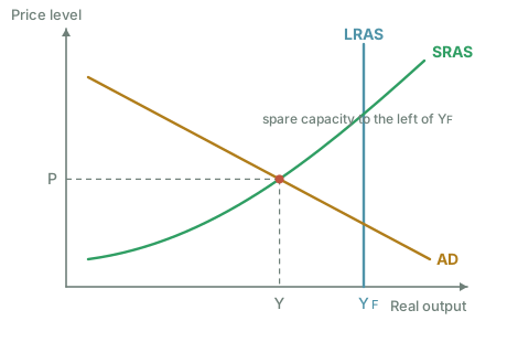
These are aggregate variables. The diagram is not the market for one product.
Central warning
Do not transfer every microeconomic demand-and-supply explanation directly into the macro model.
For example:
- AD is not demand for one good;
- AS is not supply by one firm;
- the vertical axis is the economy-wide price level, not the price of one product.
2. Aggregate demand
Definition
Aggregate demand is the total planned expenditure on domestically produced goods and services at a given general price level in a given time period.
A complete definition includes:
- total planned spending;
- domestic output;
- a given price level;
- a time period.
Formula
where:
C= consumption expenditure;I= investment expenditure;G= government expenditure on goods and services;X= exports;M= imports;X − M= net exports.
Why imports are subtracted
Consumption, investment and government-spending figures may include purchases of imported goods and services. Imports are not domestically produced output, so they must be removed.
Why exports are added
Exports are produced domestically but purchased from abroad. They are therefore part of demand for domestic output.
Government transfers are not directly part of G
Transfer payments such as pensions or unemployment benefits are not direct purchases of current output. They may influence AD indirectly when recipients spend the income, but they are not themselves counted as G in the formula.
3. Calculating aggregate demand
Worked example 1
Suppose:
- C = 620;
- I = 140;
- G = 210;
- X = 180;
- M = 230.
Then:
A trade deficit does not make AD negative. It makes the net-export component negative.
Worked example 2: change in AD
Suppose:
- C rises by 20;
- I falls by 8;
- G is unchanged;
- X rises by 5;
- M rises by 7.
Change in net exports:
Total change:
AD rises by 10.
Common calculation errors
- adding imports rather than subtracting them;
- subtracting exports;
- treating a transfer payment as a direct part of G;
- forgetting that net exports may be negative;
- confusing investment expenditure with buying shares or bonds.
4. Determinants of aggregate demand
The syllabus does not require detailed component models at AS Level. Students should nevertheless understand the principal influences on total planned spending.
4.1 Household income and employment
Higher disposable income and employment normally encourage consumption.
- Higher income/employment
- higher consumption
- AD rises.
4.2 Interest rates
Lower interest rates may:
- reduce the reward from saving;
- reduce borrowing costs;
- encourage consumption and investment.
- Lower interest rates
- C and I may rise
- AD shifts right.
The strength depends on confidence, debt and responsiveness to borrowing costs.
4.3 Consumer and business confidence
If households expect stronger future income; they may spend more. If firms expect stronger demand and profit; they may invest more.
- Higher confidence
- C and/or I rise
- AD shifts right.
4.4 Wealth
A rise in household wealth may encourage consumption, though the effect is not identical for all households or assets.
4.5 Fiscal policy
- higher government purchases directly raise G;
- lower taxes may raise disposable income and consumption;
- lower government purchases or higher taxes may reduce AD.
4.6 Monetary conditions
Changes in interest rates, money supply or credit conditions can affect consumption and investment.
4.7 Foreign income
Stronger income and output abroad may raise demand for the country's exports.
- Foreign growth
- X rises
- AD shifts right.
4.8 Exchange rate and international competitiveness
A depreciation may make exports cheaper to foreign buyers and imports more expensive to domestic buyers, tending to raise net exports and AD.
This outcome is not automatic. It depends on:
- demand elasticities;
- firms' ability to supply;
- time;
- imported input costs;
- global conditions.
4.9 Population
A larger population may increase total consumption, although the effect on living standards depends on output per person.
5. Why the AD curve slopes downward
The AD curve shows the relationship between the general price level and planned real expenditure, holding other determinants constant.
A fall in the general price level is associated with a rise in real output demanded.
5.1 Real-wealth effect
When the price level falls, the real purchasing power of money balances rises. Households may feel able to purchase more real output.
- Lower price level
- higher real value of money balances
- C rises
- greater real output demanded.
5.2 Interest-rate effect
A lower price level may reduce the amount of money needed for transactions. Under suitable monetary conditions, interest rates may fall, encouraging consumption and investment.
- Lower price level
- lower interest rates
- C and I rise
- greater real output demanded.
5.3 International-competitiveness effect
If the domestic price level falls relative to prices abroad, domestic output may become more competitive.
- Lower relative domestic price level
- X rises and M falls
- net exports rise
- greater real output demanded.
Movement along AD
A change in the general price level, with other determinants held constant, causes a movement along the AD curve.
- lower price level
- extension of aggregate demand
- higher price level
- contraction of aggregate demand.
6. Shifts in aggregate demand
A change in any non-price determinant shifts the whole AD curve.
Rightward shift
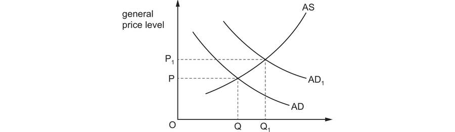
AD shifts right when planned expenditure rises at every price level.
Possible causes:
- higher consumer confidence;
- lower interest rates;
- lower direct taxes;
- higher government expenditure;
- higher business confidence;
- higher foreign income;
- improved export competitiveness;
- stronger credit availability.
Leftward shift
AD shifts left when planned expenditure falls at every price level.
Possible causes:
- lower confidence;
- higher interest rates;
- higher direct taxes;
- lower government expenditure;
- recession abroad;
- weaker competitiveness;
- tighter credit conditions.
Analysis chain
- Determinant changes
- one or more AD components change
- total planned expenditure changes
- AD shifts.
An answer that says only “confidence increases AD” is incomplete. Identify the component affected.
7. Aggregate supply
Definition
Aggregate supply is the total real output that producers in an economy are willing and able to supply at different general price levels in a given time period.
Short run versus long run
The distinction concerns adjustment.
- In the short run, some production costs and productive resources may not adjust fully.
- In the long run, wages, contracts, capacity and resource allocation have more time to adjust.
The syllabus accepts different long-run representations. Students should be able to use and interpret both accurately.
8. Determinants of aggregate supply
8.1 Resource quantity and quality
AS is affected by:
- labour-force size;
- education and skills;
- capital stock;
- quantity and quality of land and natural resources;
- entrepreneurship.
8.2 Productivity
Productivity is output per unit of input.
- Higher productivity
- lower unit cost and/or greater productive capacity
- AS increases.
8.3 Production costs
Important costs include:
- wages;
- energy;
- raw materials;
- imported inputs;
- indirect taxation;
- regulatory and financing costs.
Higher costs commonly reduce SRAS.
8.4 Technology
Better technology can raise productivity, lower unit costs and increase productive capacity.
It can therefore shift both SRAS and LRAS right, though the timing may differ.
8.5 Infrastructure
Reliable transport, communication and energy systems can improve productive efficiency and capacity.
8.6 Expectations
Expected future prices and costs can affect current supply decisions, but students should avoid vague claims. State the mechanism.
8.7 Government policy
Policies may affect:
- costs in the short run;
- productivity and capacity in the long run.
Examples include:
- indirect taxes;
- subsidies;
- education and training;
- infrastructure;
- competition policy;
- support for innovation.
8.8 Weather and supply shocks
Natural disasters, harvest failure, war or supply-chain disruption can reduce SRAS.
9. The shape of SRAS
The syllabus accepts an upward-sloping line or an upward-sweeping curve.
Why SRAS slopes upward
As the general price level rises, firms may find production more profitable when some input costs do not rise immediately or by the same proportion.
They may therefore increase real output.
As output approaches capacity:
- bottlenecks appear;
- overtime and less-efficient inputs may be required;
- unit costs rise more quickly;
- SRAS becomes steeper.
Movement along SRAS
A change in the general price level, holding supply determinants constant, causes a movement along SRAS.
- higher price level
- extension of aggregate supply
- lower price level
- contraction of aggregate supply.
10. Long-run aggregate supply: two accepted representations
10.1 Classical or vertical LRAS
The vertical LRAS curve is drawn at potential or full-employment output.
The logic is:
- the economy's sustainable real capacity depends on resources, productivity and technology;
- a change in the price level alone does not permanently change that capacity;
- in the long run, higher AD changes the price level rather than sustainable real output once full capacity is reached.
10.2 Keynesian three-section LRAS
The alternative LRAS curve contains:
- highly elastic section at low output, where substantial spare capacity allows output to rise with little price pressure;
- upward-sloping section, where bottlenecks appear and output and prices both rise;
- vertical section at full capacity, where output cannot rise further and additional AD raises only the price level.
The models are not simply “right” versus “wrong”
They emphasise different assumptions and economic conditions.
- Vertical LRAS emphasises long-run productive capacity.
- The three-section curve emphasises the degree of spare capacity and the way price pressure intensifies as full employment is approached.
Students should identify which model is being used and reason consistently from its shape.
11. Shifts in SRAS
SRAS shifts when short-run production conditions change.
SRAS shifts right
Possible causes:
- lower wage costs per unit;
- lower energy or raw-material prices;
- lower indirect taxes;
- higher production subsidies;
- improved short-run productivity;
- favourable weather;
- reduced imported-input costs.
Likely initial effect, other things equal:
- lower price level;
- higher real output;
- higher employment.
SRAS shifts left
Possible causes:
- higher wages not matched by productivity;
- higher oil or energy costs;
- higher indirect taxes;
- currency depreciation raising imported-input costs;
- natural disaster;
- supply-chain disruption;
- lower short-run productivity.
Likely initial effect, other things equal:
- higher price level;
- lower real output;
- lower employment.
This combination is commonly called stagflation when falling or stagnant output occurs alongside inflation.
12. Shifts in LRAS
LRAS shifts when the economy's productive capacity changes.
LRAS shifts right
Possible causes:
- larger or more skilled labour force;
- increased capital stock;
- technological progress;
- improved education and training;
- better infrastructure;
- discovery or improved use of resources;
- stronger productivity;
- improved institutions that raise productive potential.
A rightward shift represents an increase in potential output.
LRAS shifts left
Possible causes:
- destruction of capital;
- loss of productive labour;
- long-lasting decline in skills or productivity;
- depletion or loss of usable resources;
- severe institutional breakdown.
Important distinction
A temporary fall in current output does not necessarily shift LRAS left.
Example:
A short recession may reduce actual output without immediately reducing the economy's potential capacity.
13. Movement versus shift
| Curve | Movement along curve | Shift of curve |
|---|---|---|
| AD | Change in general price level | Change in C, I, G or net exports caused by a non-price determinant |
| SRAS | Change in general price level | Change in short-run production costs or conditions |
| LRAS | Normally not analysed as a standard movement response in the vertical model | Change in productive capacity |
Exam trap
A rise in the price level does not itself shift AD or SRAS. It causes movement along the relevant curve, provided other determinants are unchanged.
14. Macroeconomic equilibrium
Equilibrium occurs where aggregate demand equals aggregate supply.
At the intersection, the model determines:
- equilibrium real output;
- equilibrium price level.
Employment
Employment is not usually read from a separate axis. It is inferred from real output and productive conditions.
General chain:
- Higher real output
- firms require more labour
- employment tends to rise
- cyclical unemployment tends to fall.
Qualification:
- productivity changes can alter the labour needed per unit of output;
- firms may change hours before worker numbers;
- labour-market frictions affect the speed of adjustment;
- the economy may already be close to full employment.
Disequilibrium and adjustment
If planned aggregate expenditure is inconsistent with current output and prices, firms experience inventory changes and adjust production, prices and employment. The exact process depends on the model and time period.
15. Effects of a rightward shift in AD
Assume AD rises because one or more expenditure components rise.
With substantial spare capacity
Likely effects:
- real output rises significantly;
- employment rises;
- price level rises little or moderately.
Near full capacity
Likely effects:
- real output rises only slightly or not at all;
- employment has limited scope to rise;
- price level rises strongly.
Vertical LRAS case
In the long-run vertical model, a permanent rightward AD shift changes the price level but not potential real output.
Conditional chain
- AD rises
- firms receive more orders
- inventories fall
- firms raise output and employment where spare capacity exists
- bottlenecks intensify as capacity is approached
- price pressure rises.
16. Effects of a leftward shift in AD
Likely short-run effects:
- lower real output;
- lower employment;
- lower price level or slower inflation.
If prices and wages adjust slowly, the fall in output and employment may be substantial.
A leftward AD shift can create cyclical unemployment.
17. Effects of a rightward shift in AS
SRAS right
Likely effect:
- real output rises;
- price level falls;
- employment rises.
This is a favourable short-run supply change.
LRAS right
Productive capacity rises.
Potential implications:
- greater sustainable output;
- greater scope for employment;
- lower inflationary pressure at a given AD;
- economic growth in potential output.
The actual equilibrium result also depends on AD.
18. Effects of a leftward shift in AS
SRAS left
Likely effect:
- real output falls;
- employment falls;
- price level rises.
This creates a difficult policy trade-off even though formal policy conflicts are developed later.
LRAS left
Potential output falls. The economy can sustainably produce less.
Possible consequences:
- lower real output;
- higher price pressure for a given level of AD;
- reduced employment capacity;
- lower living standards.
19. Simultaneous shifts
Real economies often experience more than one change.
AD right and AS right
- real output definitely rises;
- price-level effect is ambiguous.
AD left and AS left
- real-output effect is generally downward;
- price-level effect is ambiguous because both shifts affect price in opposite directions.
AD right and AS left
- price level definitely rises;
- output effect is ambiguous.
AD left and AS right
- price level definitely falls;
- output effect is ambiguous.
A strong answer states what is certain and what depends on relative shift size.
20. Employment analysis
Employment effects should follow output analysis rather than be asserted mechanically.
Demand-side expansion
If spare capacity and unemployed labour exist:
- AD right
- real output rises
- derived demand for labour rises
- employment rises.
Near full employment:
- AD right
- output changes little
- price level rises strongly
- employment changes little.
Positive supply-side change
- AS right
- firms can produce more at lower unit cost
- output rises
- labour demand may rise.
But if the shift is caused by labour-saving technology, output may rise without an equal rise in employment. The effect depends on whether expansion of output outweighs the reduction in labour required per unit.
21. Applying the model accurately
Example 1: consumer confidence rises
- Households increase planned consumption.
- C rises.
- AD shifts right.
- Output and employment rise if spare capacity exists.
- The price level rises, especially near capacity.
Example 2: oil prices rise
- Energy and transport costs rise.
- Unit production costs rise.
- SRAS shifts left.
- Real output and employment fall.
- The price level rises.
Example 3: workforce skills improve
- Labour productivity and productive potential rise.
- LRAS shifts right.
- Sustainable real output increases.
- Inflationary pressure at a given AD is reduced.
- Actual output rises only if sufficient demand exists.
Example 4: recession abroad
- Foreign income falls.
- Demand for exports falls.
- X falls.
- AD shifts left.
- Domestic output and employment fall; price pressure weakens.
Example 5: currency depreciation
Possible AD effect:
- exports become more competitive;
- imports become more expensive;
- net exports may rise;
- AD may shift right.
Possible AS effect:
- imported input costs rise;
- SRAS may shift left.
Therefore the price level is likely to rise, while the output effect may be ambiguous.
22. Common misconceptions and exam traps
Trap 1: AD is simply consumer demand
Wrong. AD includes C, I, G and net exports.
Trap 2: Imports are added
Wrong. Imports are subtracted because they are not domestic output.
Trap 3: Transfer payments are directly part of G
Wrong. They are not purchases of current output.
Trap 4: Investment means buying financial assets
Wrong in the AD identity. Investment means expenditure on capital goods and related additions to productive capacity or inventories.
Trap 5: A price-level change shifts AD
Wrong. It causes movement along AD.
Trap 6: A higher price level shifts SRAS
Wrong. It causes movement along SRAS.
Trap 7: Higher AD always raises real output by the same amount
Wrong. The result depends on spare capacity and the shape of AS.
Trap 8: Higher AD always reduces unemployment greatly
Wrong near full employment or where supply constraints dominate.
Trap 9: A temporary recession necessarily shifts LRAS left
Wrong. Actual output can fall while potential output is unchanged.
Trap 10: SRAS and LRAS have the same determinants
Some influences overlap, but short-run cost changes need not alter long-run capacity.
Trap 11: Any technology improvement automatically raises employment
Wrong. It raises productive potential, but the employment effect depends on output expansion and labour-saving effects.
Trap 12: The two LRAS representations contradict each other completely
They emphasise different assumptions. Use the model specified or shown.
Trap 13: A rightward AS shift always means zero inflation
It reduces price pressure relative to what otherwise would occur. AD can still rise enough to increase the price level.
Trap 14: Simultaneous shifts always give a definite result for both axes
Often one outcome is ambiguous.
23. Paper 1 technique
Typical tasks include:
- identify an AD component;
- calculate AD;
- classify a determinant as affecting AD, SRAS or LRAS;
- distinguish movement and shift;
- interpret a change in equilibrium;
- identify which variable is certain under simultaneous shifts;
- link output to employment conditionally.
Six-step method
- Identify the initial curve affected.
- State the direction of the shift.
- Explain the determinant and mechanism.
- Identify the new equilibrium output.
- Identify the new price level.
- Infer the employment effect with a qualification where needed.
24. Paper 2 technique
Four-mark definition and component question
Aggregate demand is total planned expenditure on domestically produced goods and services at a given price level in a given period. It equals consumption, investment and government expenditure plus exports minus imports.
Six-mark AD-shift question
A fall in interest rates may lower borrowing costs and reduce the reward from saving. Consumption and investment may rise, increasing total planned expenditure. AD therefore shifts right. With spare capacity, real output and employment rise, while the price level also rises. The output effect is weaker and the price effect stronger near full capacity.
Eight-mark supply-shock question
A rise in energy prices increases firms' unit costs and shifts SRAS left. At the new equilibrium, the price level is higher while real output and employment are lower. The size depends on the elasticities or shapes of AD and AS, the importance of energy in costs and whether firms can substitute other inputs.
Twelve-mark discussion
Question:
Discuss whether an increase in aggregate demand will always improve an economy's macroeconomic performance.
Analysis in favour:
- raises real output where spare capacity exists;
- raises employment and income;
- may improve business confidence and investment.
Evaluation:
- near full capacity it mainly raises prices;
- higher imports may weaken net exports;
- labour or infrastructure bottlenecks limit output;
- effects depend on cause, size and duration;
- supply-side conditions matter;
- short-run gain may differ from long-run result.
Judgement:
An AD increase is most likely to improve output and employment when substantial spare capacity exists and SRAS is responsive. Close to full capacity, the main effect is likely to be inflation rather than a sustained rise in real output.
25. Active recall
- Define aggregate demand.
- State and explain the AD formula.
- Why are imports subtracted?
- Why are exports added?
- Why are transfer payments not directly included in G?
- Give four determinants of AD.
- Explain three reasons why AD slopes downward.
- Distinguish movement along AD from a shift.
- Define aggregate supply.
- Give five determinants of AS.
- Explain why SRAS slopes upward.
- Describe the vertical LRAS model.
- Describe the three-section LRAS model.
- Give four causes of an SRAS rightward shift.
- Give four causes of an LRAS rightward shift.
- Distinguish a temporary fall in actual output from a fall in potential output.
- Define macroeconomic equilibrium.
- How is employment inferred from the model?
- Explain a rightward AD shift with spare capacity.
- Explain a rightward AD shift near full capacity.
- Explain a leftward SRAS shift.
- Explain a rightward LRAS shift.
- What is certain when AD shifts right and AS shifts left?
- Why may currency depreciation shift both AD and SRAS?
- Why does higher output not always produce a proportionate employment rise?
26. One-minute revision summary
AD
- downward sloping;
- price-level change
- movement along
- non-price spending change
- shift.
AS
- SRAS usually slopes upward;
- LRAS may be vertical or shown in three sections;
- short-run cost change
- SRAS shift
- productive-capacity change
- LRAS shift.
Equilibrium
AD and AS determine:
- real output;
- general price level;
- employment indirectly through output and labour demand.
Core conditional result
More AD raises output and employment most when spare capacity exists; near full capacity it mainly raises the price level.
Check you have it
Question 1
The diagram shows the original aggregate demand curve, AD1, and original aggregate supply curve, AS1. The original equilibrium is at X. AS1 AS2 AD1 Y1 Y2 P2 P1 O price level real GDP Y X What would cause the new equilibrium to be at Y?
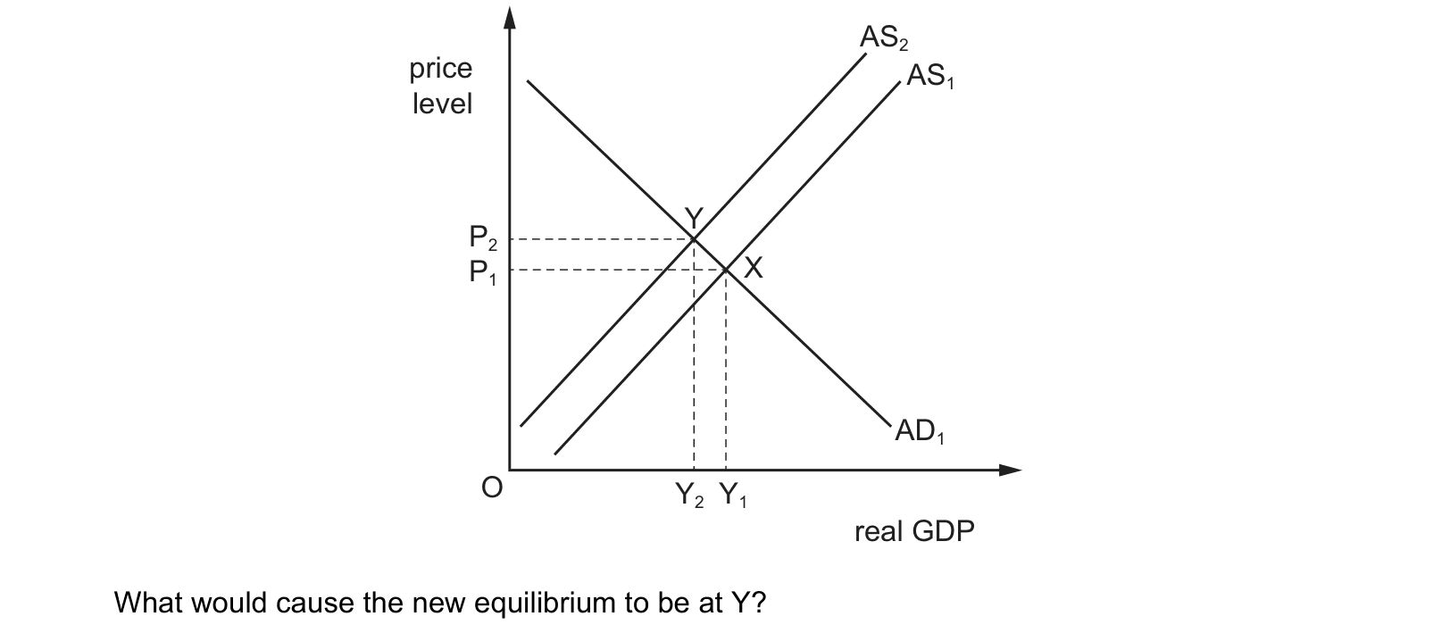
Answer: C.
Question 2
The diagram shows an economy with an initial equilibrium real output of Y1 at a price level of P1. price level real output O AS1 AD1 Y1 P1 Y2 AS2 AD2 Which combination of events is likely to cause the equilibrium real output to rise to Y2?
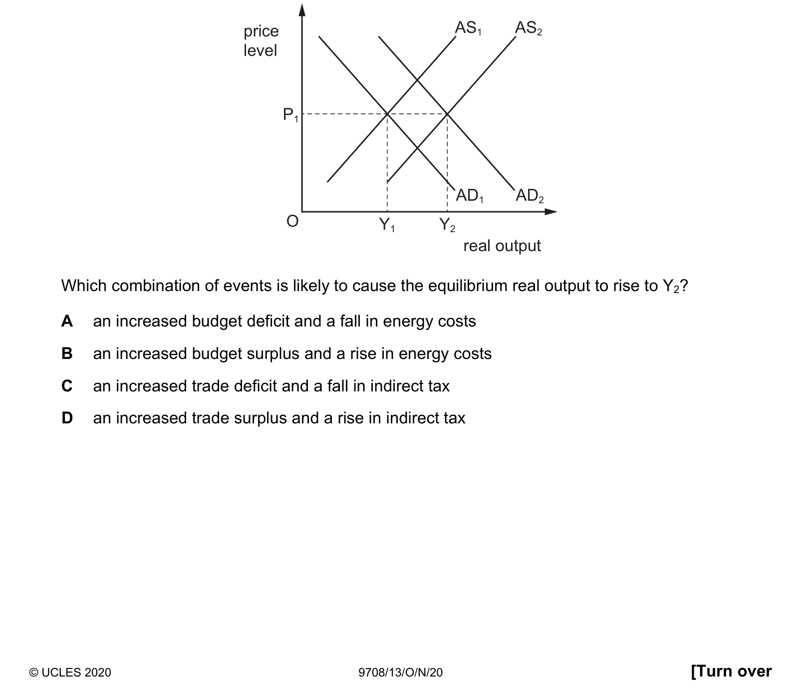
Answer: A.
Explanation:
1. Increased budget deficit: When the government increases its budget deficit, it injects more money into the economy through increased government spending. This increase in government spending will lead to higher aggregate demand (AD), shifting the AD curve to the right. As a result, the equilibrium real output will increase from Y1 to Y2.
2. Fall in energy costs: A fall in energy costs will lead to a decrease in production costs for firms. Lower production costs will lead to an increase in supply (shift the AS curve to the right), allowing firms to produce more output at lower prices. This will lead to an increase in equilibrium real output from Y1 to Y2.
Combining these two factors (increased budget deficit and a fall in energy costs) will lead to an overall increase in equilibrium real output (Y2) in the economy.
Therefore, option A is the correct choice as it provides a combination of events that are likely to cause the equilibrium real output to rise to Y2.
Question 3
An aggregate demand curve slopes downwards from left to right. One reason for this is that a reduction in the average price level will lead to
Answer: C.
Explanation:
An aggregate demand (AD) curve shows the relationship between the aggregate quantity of goods and services demanded in an economy at different price levels. The downward slope of the AD curve is due to the wealth effect and the interest rate effect.
- The wealth effect: A decrease in the average price level increases the purchasing power of consumers (real value of money balances), making them feel wealthier. As a result, consumers are more likely to spend money on goods and services, leading to an increase in aggregate demand.
- The interest rate effect: When the price level decreases, the real value of money balances increases. This increase in real money balances leads to a lower demand for money, causing interest rates to fall. Lower interest rates encourage more borrowing and investment, further boosting aggregate demand.
Let's analyse the other options:
A - A reduction in the average price level will not lead to a decline in the country's international competitiveness. In fact, a decrease in average price levels can make a country's exports more competitive in international markets, potentially boosting aggregate demand.
B - A decrease in the average price level will not directly lead to an increase in interest rates. On the contrary, as explained earlier, a decrease in price levels will likely lead to a decrease in interest rates due to the interest rate effect.
D - The expectation of further price falls may influence individual consumption decisions but does not directly explain the downward slope of the aggregate demand curve.
Diagram policy
No rendered AD/AS graph in this content pack is authorised for publication. Use the audited written specifications only until an economics expert verifies all curve positions, shifts, labels and equilibrium outcomes.
What the syllabus asks for on this topicOfficial syllabus coverage · Product mastery map
Official syllabus coverage
Students must understand:
- 4.3.1 the definition of Aggregate Demand (AD);
- 4.3.2 the components and meanings of
AD = C + I + G + (X − M); - 4.3.3 determinants of AD, without detailed component theory;
- 4.3.4 why the aggregate demand curve (AD curve) slopes downward;
- 4.3.5 causes of shifts in AD;
- 4.3.6 the definition of Aggregate Supply (AS);
- 4.3.7 determinants of AS;
- 4.3.8 the shape of SRAS and the two accepted LRAS representations;
- 4.3.9 causes of shifts in SRAS and LRAS;
- 4.3.10 movements along versus shifts of AD and AS;
- 4.3.11 macroeconomic equilibrium and determination of real output, the price level and employment;
- 4.3.12 effects of AD and AS shifts on real output, the price level and employment.
Product mastery map
The portal tracks one skill for each syllabus requirement:
- AD definition;
- AD components;
- AD determinants;
- downward-sloping AD;
- AD shifts;
- AS definition;
- AS determinants;
- SRAS and LRAS shapes;
- SRAS and LRAS shifts;
- movement versus shift;
- equilibrium and employment;
- effects of AD and AS changes.

Related CIE 9708 topics
Not the topic you were looking for? Describe what you are stuck on in your own words and we will take you to the notes that answer it.