Labour Market Forces and Government Intervention
Wage Determination, Trade Unions, Monopsony and Labour Market Policy
Contents: 11 sections
1. Why this topic matters
The labour market is where most people's income is decided, so it links directly to 8.2 on equity. It is also the topic where CIE most often rewards a candidate who can apply ordinary demand and supply analysis to a market with unusual features.
The analytical core is simple to state and easy to get wrong: labour is demanded not for itself but for what it produces. Demand for labour is a derived demand. A firm hires a worker because that worker adds to revenue, so anything that changes the value of what the worker produces changes the demand for that worker.
Three results carry most of the marks in this topic:
- the wage in a competitive labour market is set by the interaction of market demand and market supply, and the individual firm is a wage taker;
- a monopsony employer pays less than the competitive wage and hires fewer workers; and
- because of that, a trade union or a minimum wage can raise both wages and employment in a monopsony, which reverses the competitive prediction.
A candidate who knows only the competitive case will assert that minimum wages always cause unemployment and will lose evaluation marks every time.
2. The demand for labour
2.1 Marginal revenue product
The marginal revenue product of labour (MRPL) is the addition to a firm's total revenue from employing one more worker.
MRPL equals the marginal physical product of labour (MPPL) multiplied by the marginal revenue from selling that output.
For a firm selling in a perfectly competitive product market, price equals marginal revenue, so MRPL equals MPPL multiplied by price.
2.2 Why the MRPL curve slopes downward
MRPL falls as more workers are hired for two reasons, and both should be named:
- diminishing returns: with at least one fixed factor, each extra worker eventually adds less physical output than the last, so MPPL falls; and
- falling marginal revenue: where the firm faces a downward sloping demand curve for its product, selling extra output requires a lower price, so marginal revenue falls too.
In perfect competition only the first reason applies. In imperfect competition both do, so the MRPL curve falls more steeply.
2.3 The profit maximising level of employment
A firm hires up to the point where MRPL equals the marginal cost of labour (MCL).
- If MRPL exceeds MCL, the extra worker adds more to revenue than to cost, so hiring raises profit.
- If MCL exceeds MRPL, the last worker reduces profit, so the firm should hire fewer.
For a firm in a competitive labour market, the marginal cost of labour is simply the wage, so the rule becomes hire where MRPL equals the wage. The MRPL curve is therefore the firm's labour demand curve.
2.4 Worked calculation
A firm sells output at a fixed price of $8. Labour is the only variable factor.
| Workers | Total product | Marginal product | MRPL at $8 |
|---|---|---|---|
| 1 | 12 | 12 | $96 |
| 2 | 26 | 14 | $112 |
| 3 | 38 | 12 | $96 |
| 4 | 46 | 8 | $64 |
| 5 | 50 | 4 | $32 |
If the market wage is $64, the firm employs 4 workers, because the fourth adds $64 to revenue and costs $64, while a fifth would add only $32.
If the wage falls to $32, the firm employs 5. This traces out the downward sloping demand curve for labour.
Note that diminishing returns begin after the second worker, where marginal product first falls, not where MRPL first falls below the wage.
2.5 Shifts in the demand for labour
The demand curve shifts when anything other than the wage changes MRPL:
- a change in the price of the product, since MRPL depends on it directly;
- a change in labour productivity, through training, better technology or improved management;
- a change in the price of substitute factors, such as cheaper automation reducing labour demand;
- a change in demand for the final product, since labour demand is derived; and
- non-wage employment costs such as social contributions.
2.6 Elasticity of demand for labour
Demand for labour is more elastic when:
- labour is a large proportion of total cost, so a wage rise matters more;
- substitutes such as machinery are readily available;
- demand for the final product is price elastic; and
- the time period is longer, since capital can be substituted.
This elasticity determines how much employment falls when wages rise, so it is central to evaluating both trade unions and minimum wages.
3. The supply of labour
3.1 Supply to an occupation
The supply of labour to a particular occupation rises with the wage, because a higher relative wage attracts workers from other occupations.
Supply shifts with:
- the wage in alternative occupations;
- qualification and training requirements, which restrict entry;
- non-monetary characteristics: danger, status, hours, location, job security;
- the size and skills of the working population, including migration; and
- barriers such as professional licensing or union membership rules.
3.2 Elasticity of labour supply
Supply is more inelastic where training is long and specialised, as in surgery, and more elastic where the work requires little specific training. This is why high demand for an inelastically supplied talent produces very high pay, which links directly to inequality in 8.2.
3.3 The backward bending supply curve for an individual
For an individual, a higher wage has two opposing effects:
- the substitution effect: leisure becomes more expensive in terms of income forgone, so the worker substitutes work for leisure and supplies more hours; and
- the income effect: the worker can reach a target income with fewer hours, and if leisure is a normal good, demand for leisure rises, so hours supplied fall.
At low wages the substitution effect dominates and supply slopes upward. At high wages the income effect may dominate, and the curve bends backwards.
This applies to an individual. The market supply curve normally still slopes upward, because higher wages attract new entrants to the occupation.
4. Wage determination in a competitive labour market
In a perfectly competitive labour market there are many buyers and sellers of labour, labour is homogeneous, there is perfect information, and there is freedom of entry and exit.
The market wage is set where market demand equals market supply. The individual firm is a wage taker: it faces a perfectly elastic supply of labour at that wage, so average cost of labour equals marginal cost of labour equals the wage. It hires where MRPL equals that wage.
Wage differentials between occupations then arise from differences in demand, reflecting productivity, and differences in supply, reflecting training requirements and non-monetary factors.
5. Monopsony
5.1 The structure
A monopsony is a labour market with a single, or dominant, buyer of labour. Examples include a state health service employing nurses, or a single large employer in an isolated town.
The monopsonist faces the upward sloping market supply curve of labour. To hire an additional worker it must raise the wage, and, where it cannot discriminate; it must pay that higher wage to all its existing workers.
5.2 Why marginal cost of labour exceeds the wage
Because raising the wage for one extra worker raises it for everyone already employed, the marginal cost of an extra worker is the new wage plus the increase paid to all existing staff. The MCL curve therefore lies above the supply curve and rises more steeply.
Worked example. Supply is such that 10 workers require a wage of $200 and 11 workers require $210.
- Total wage bill at 10 workers: $2,000.
- Total wage bill at 11 workers: 11 multiplied by $210 equals $2,310.
- Marginal cost of the 11th worker: $310, not $210.
The extra $100 is the $10 rise paid to each of the 10 existing workers.
5.3 The outcome
The monopsonist hires where MRPL equals MCL, then reads the wage it must pay off the supply curve at that quantity, which is lower than MRPL at that point.
Compared with the competitive outcome, a monopsonist employs fewer workers at a lower wage. There is a welfare loss, and workers are paid less than the value of what they produce, which is a form of exploitation in the technical sense.
6. Trade unions
6.1 What a union does
A trade union is an organisation of workers acting collectively to improve pay and conditions. Through collective bargaining it acts as a monopoly seller of labour.
A union may raise wages by:
- bargaining directly for a wage above the equilibrium, which makes supply perfectly elastic at the negotiated wage up to the number willing to work;
- restricting supply through entry requirements, apprenticeship control or closed shop arrangements; and
- raising the demand for labour, by supporting productivity improvements or campaigning for protection of the industry.
6.2 The competitive case
In an otherwise competitive labour market, a union that raises the wage above equilibrium creates excess supply of labour. Employment falls, and those still employed gain at the expense of those who lose their jobs or cannot enter.
The size of the employment loss depends on the elasticity of demand for labour. Where demand is inelastic, because labour is a small share of cost or has few substitutes, the union can achieve a large wage gain for a small employment loss.
6.3 The monopsony case
Where the employer is a monopsonist, a union can raise both the wage and employment.
By setting a wage floor, the union makes labour supply perfectly elastic at that wage up to the number willing to work. The employer can no longer depress the wage by restricting hiring, so the marginal cost of labour equals the negotiated wage over that range. The employer then hires where MRPL equals that wage, which is more workers than before.
This is bilateral monopoly: a monopoly seller facing a monopsony buyer. The outcome lies between the two extremes and depends on relative bargaining power, so theory cannot predict a unique wage. Saying so explicitly is a strong evaluation point.
6.4 Evaluation of union power
Union effectiveness depends on:
- the elasticity of demand for labour;
- the proportion of the workforce in membership;
- the profitability of the firm and its ability to pay;
- legal restrictions on industrial action; and
- whether the employer can relocate or automate.
Unions may also raise productivity by giving workers a collective voice, reducing turnover and improving training, which shifts MRPL rightward and offsets the employment cost.
7. Government intervention in the labour market
7.1 National minimum wage
A minimum wage is a price floor. Its effects follow directly from the two cases above:
- in a competitive market, it causes excess supply and reduces employment, with the loss larger where labour demand is elastic; and
- in a monopsony; it can raise employment as well as pay.
Further evaluation:
- it raises the incomes of the low paid and may reduce the poverty trap by making work pay;
- but it does not target poor households, since some low paid workers are second earners in higher income households;
- it may raise costs and prices, so real gains are smaller than nominal ones;
- it may push activity into the informal economy where enforcement is weak; and
- it may compress differentials and prompt higher paid workers to seek restoration, causing a wage price spiral.
7.2 Maximum wages
A maximum wage is a ceiling, occasionally proposed for executive pay. It would reduce inequality directly but may cause an outflow of talent, avoidance through non-wage remuneration, and shortages in affected occupations.
7.3 Policies to improve labour market outcomes
- Education and training raise MPPL and therefore MRPL, shifting labour demand rightward and raising both wages and employment. This is the only policy that raises pay without an employment cost, but it is slow.
- Improving labour mobility: occupational mobility through retraining, and geographical mobility through housing and transport policy, both reduce structural unemployment.
- Anti-discrimination legislation widens the occupations open to affected groups, raising their wages.
- Improving information about vacancies reduces frictional unemployment.
- Trade union legislation can strengthen or weaken bargaining power depending on its direction.
8. Transfer earnings and economic rent
Syllabus point 8.3.10, and a reliable source of marks because the two terms are easy to define and easy to confuse.
8.1 The definitions
Transfer earnings are the minimum payment necessary to keep a factor of production in its present use. They are the factor's opportunity cost: what it could earn in its next best alternative.
Economic rent is any payment received above transfer earnings. It is a surplus, in the sense that the factor would have supplied its services without it.
Actual earnings = transfer earnings + economic rent
8.2 A worked case
A software engineer earns $90,000. Her next best alternative, teaching mathematics, would pay $45,000, and she would take the engineering job at anything above that.
- Transfer earnings = $45,000, the amount required to stop her transferring to teaching.
- Economic rent = 90,000 − 45,000 = $45,000.
Note that transfer earnings are specific to the individual and to the alternative available. A colleague with no teaching qualification, whose next best option pays $30,000, has higher economic rent at the same salary.
8.3 Reading it from the diagram
On a labour market diagram, at the equilibrium wage:
- Transfer earnings are the area under the supply curve up to the equilibrium quantity, because the supply curve shows the minimum each successive worker would accept.
- Economic rent is the area between the wage line and the supply curve, since every worker except the marginal one is paid more than their minimum.
Only the last worker hired earns no economic rent, because for that worker the wage exactly equals their transfer earnings.
8.4 What determines the split
The division depends on the elasticity of supply of labour to the occupation.
- Inelastic supply means a large proportion is economic rent. Supply is inelastic where the skill takes years to acquire, where talent is scarce and cannot be reproduced by training, or where entry is restricted by qualification requirements. Elite footballers and surgeons earn very large economic rents on this reasoning.
- Elastic supply means a large proportion is transfer earnings. Supply is elastic where the work requires little specific training, so workers can move in easily from other occupations.
- Perfectly elastic supply means earnings are entirely transfer earnings and economic rent is zero.
- Perfectly inelastic supply means earnings are entirely economic rent, which is the case usually applied to land in a fixed location.
Time matters too. Supply is more elastic in the long run, because workers can train and relocate, so economic rent in a well-paid occupation tends to be eroded as entrants arrive. That erosion is the labour market equivalent of entry competing away supernormal profit in 7.6.
8.5 Why it is examined
Economic rent explains wage differentials that a simple demand-and-supply story leaves unexplained: two occupations with similar demand can pay very differently if one has far more inelastic supply. It also underlies the argument that taxing economic rent does not reduce the quantity supplied, since by definition the factor would have worked without it, which is a point Cambridge rewards when it appears in a question about taxing high incomes.
9. Integrated analysis and common traps
8.1 A complete chain
A government raises the minimum wage in a region dominated by one large employer. Because the employer is a monopsonist, the marginal cost of labour previously exceeded the wage, and employment was below the competitive level. The wage floor removes the employer's ability to restrict hiring to hold pay down, so MCL equals the new wage over the relevant range and employment rises. Whether this holds depends on the floor being set no higher than the MRPL at the competitive quantity; set above that, the standard excess supply result returns.
8.2 Common examination errors
- Asserting that a minimum wage always reduces employment without identifying market structure.
- Confusing marginal physical product with marginal revenue product.
- Drawing MCL below the supply curve for a monopsonist, or equal to it.
- Reading the monopsony wage off the MRPL curve rather than the supply curve.
- Saying diminishing returns begin where MRPL falls below the wage rather than where marginal product first falls.
- Treating the individual's backward bending supply curve as the market supply curve.
- Forgetting that demand for labour is derived, so a fall in product demand reduces labour demand regardless of the wage.
10. Paper 3 and Paper 4 mastery
Paper 3 tests: calculating MRPL from a product table and a price, identifying the profit maximising number of workers, computing marginal cost of labour under monopsony, and identifying the direction of a shift in labour demand.
Paper 4 essays repeatedly ask whether unions or minimum wages benefit workers. The high scoring structure is: set out the competitive result, then the monopsony result, then state which applies under what conditions, and reach a judgement that names the condition. Elasticity of labour demand is the variable that most often decides the answer, so make it explicit.
Check you have it
Question 1
What is the essential feature of nudge theory?
Answer: D.
Nudge theory comes from behavioural economics and works by changing how choices are presented rather than by removing or repricing them. It relies on persuasion and on exploiting predictable features of human decision-making, the pull of defaults, the power of social comparison, the salience of vivid information. Crucially it preserves freedom of choice: the individual can always ignore the nudge, which is why the approach is sometimes called libertarian paternalism.
Why the other options are wrong:
- B, establishing a legal requirement, is regulation. It removes options by compulsion, which is the opposite of a nudge.
- A, satisficing, is an objective a firm might pursue, settling for a satisfactory rather than a maximum outcome. It is a behavioural idea, which makes it tempting, but it describes how decisions are made rather than how a policymaker influences them.
- C, a contestable market, is a market structure defined by free entry and exit. It has nothing to do with behavioural intervention.
Question 2
A country’s government banned cigarette smoking in enclosed public spaces, such as offices, shops, bars and restaurants.
What is a government failure arising from this ban?
Answer: C.
Government failure means intervention producing an outcome that was not intended and that reduces welfare. Banning smoking indoors pushed smokers onto pavements and doorways, and the discarded cigarette ends became a new litter and street-cleaning problem, a negative externality created by the policy itself. The ban addressed one externality, passive smoking indoors, and generated another outdoors. Local authorities now bear cleaning costs they did not previously face.
Why the other options are wrong:
- A, reduced cigarette consumption, is an intended benefit. Reducing consumption of a demerit good is a goal of the policy, not a failure.
- B, reduced passive smoking, is the ban's primary objective, protecting non-smokers from an externality imposed on them. It is the clearest measure of success.
- D, higher sales of nicotine patches and gum, is a beneficial side effect: smokers substituting towards less harmful alternatives is exactly what public health policy wants.
Question 3
The table shows the average incomes of the richest 20% of households and the poorest 20% of households in the UK (2015–2016), and the effects of government taxation and benefits on average income. The two columns give the average income (£) of the richest 20% and of the poorest 20%. What can be concluded from the information in the table?
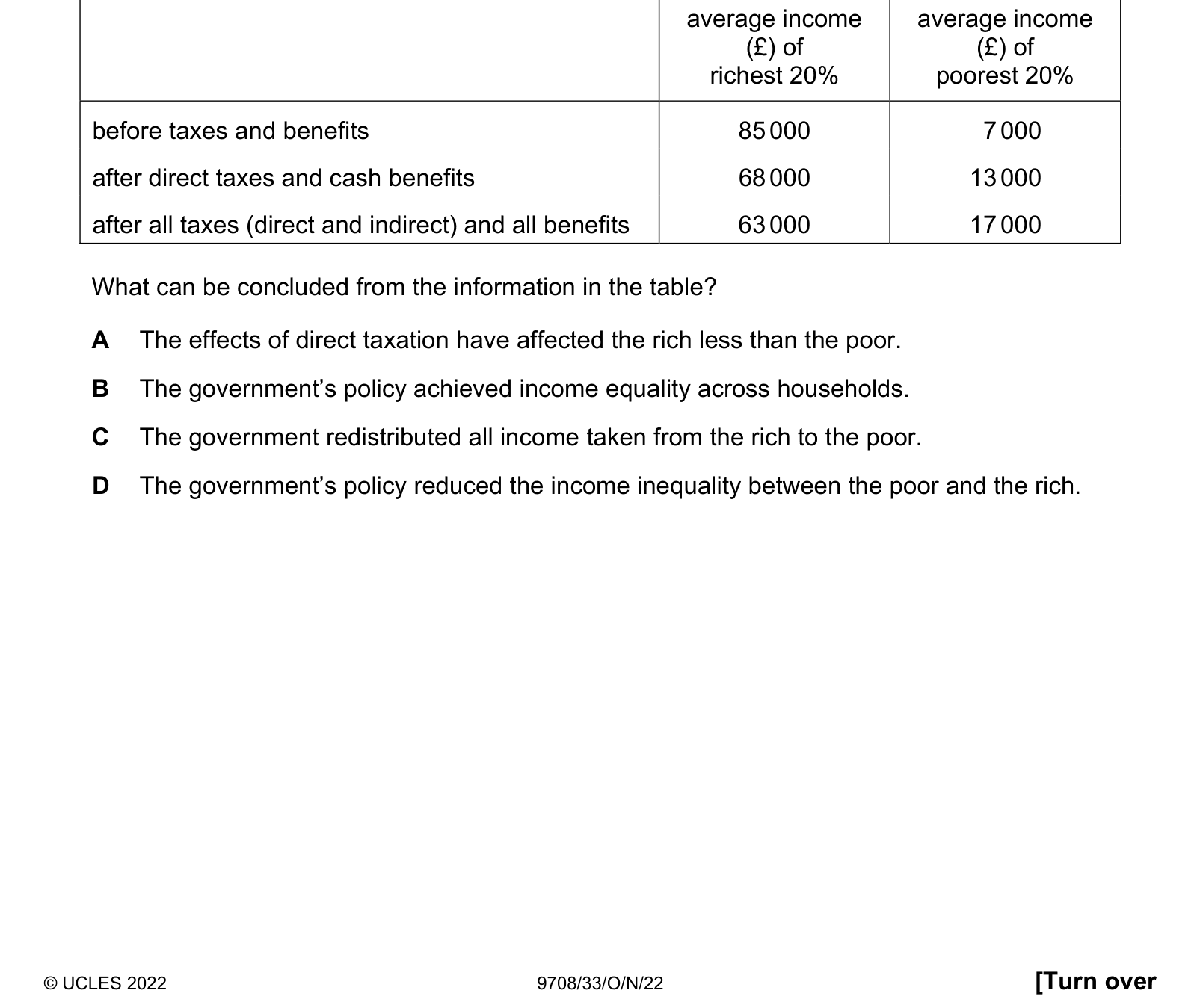
Answer: D.
11. Final checklist
A fully prepared learner can:
- explain why demand for labour is derived and what follows from that;
- define MRPL and calculate it from a product table and product price;
- explain both reasons why MRPL slopes downward and say which applies in perfect competition;
- apply the MRPL equals MCL hiring rule and identify employment at a given wage;
- list the determinants of labour demand and supply and of their elasticities;
- explain the substitution and income effects behind a backward bending individual supply curve;
- explain why MCL lies above the supply curve under monopsony, with a numerical example;
- show that a monopsonist employs fewer workers at a lower wage than a competitive market;
- explain how a union or minimum wage can raise employment under monopsony;
- explain bilateral monopoly and why theory gives no unique wage; and
- evaluate minimum wage policy using elasticity, targeting, informality and differentials.
Related CIE 9708 topics
Not the topic you were looking for? Describe what you are stuck on in your own words and we will take you to the notes that answer it.