Price, Income and Cross Elasticities of Demand
Contents: 24 sections
Topic overview
Elasticity measures responsiveness.
Demand may respond to:
- a change in the product's own price: PED;
- a change in consumer income: YED;
- a change in the price of another product: XED.
The formulas look similar, but the denominator and interpretation differ.
1. Percentage change
Elasticity compares relative percentage changes, not absolute changes.
Standard percentage-change formula
Percentage change = (change / original value) × 100
Example:
Price rises from $20 to $25.
- change = $5;
- original price = $20;
- percentage change = 5 / 20 × 100 = 25%.
Quantity demanded falls from 100 to 80.
- change = −20;
- original quantity = 100;
- percentage change = −20 / 100 × 100 = −20%.
Why percentages matter
A fall of 10 units is large if the original quantity was 20, but small if the original quantity was 10 000.
Elasticity standardises the changes so responsiveness can be compared across:
- products;
- countries;
- currencies;
- time periods;
- units of measurement.
Examination rule
Use the starting value as the denominator unless the question explicitly provides or requests another method.
Show working. A correct formula without percentage changes is incomplete when a question asks for the formula.
Cambridge calculation convention
The syllabus requires formulae and calculations but does not prescribe the midpoint/arc-elasticity method. Unless a question explicitly states another method, calculate percentage change from the original value. The word “midpoint” elsewhere in this topic refers to the middle of a straight-line demand curve, where PED is unit elastic; it is not a required calculation method.
2. Price elasticity of demand (PED)
Definition
Price elasticity of demand measures the responsiveness of quantity demanded to a change in the product's own price, ceteris paribus.
Formula
PED = percentage change in quantity demanded / percentage change in price
Sign
For a normal downward-sloping demand curve:
- price and quantity demanded move in opposite directions;
- the PED coefficient is therefore normally negative.
When describing whether demand is elastic or inelastic, economists commonly use the absolute magnitude of PED.
Example:
- PED = −2 has magnitude 2 and is elastic;
- PED = −0.4 has magnitude 0.4 and is inelastic.
A strong exam answer can state both:
PED is −2; its absolute value is greater than 1, so demand is elastic.
PED calculation example
Price rises from $10 to $12. Quantity demanded falls from 500 to 400.
Percentage change in price:
2 / 10 × 100 = +20%
Percentage change in quantity demanded:
−100 / 500 × 100 = −20%
PED:
−20% / +20% = −1
Demand is unit elastic over this price change.
Relative percentage interpretation
PED compares the percentage response in quantity demanded with the percentage change in price.
- quantity changes by a larger percentage than price
- elastic
- quantity changes by the same percentage as price
- unit elastic
- quantity changes by a smaller percentage than price
- inelastic.
3. PED coefficient values
Perfectly inelastic demand
PED = 0
Quantity demanded does not change when price changes.
Diagram:
- vertical demand curve.
Pure examples are rare. A life-saving drug with no alternative may be highly inelastic, but not necessarily perfectly inelastic over every price range.
Inelastic demand
0 < |PED| < 1
Quantity demanded changes by a smaller percentage than price.
Example:
- price rises 10%;
- quantity demanded falls 4%;
- PED = −0.4.
Unit elastic demand
|PED| = 1
Quantity demanded changes by the same percentage as price.
Elastic demand
|PED| > 1
Quantity demanded changes by a larger percentage than price.
Example:
- price falls 5%;
- quantity demanded rises 15%;
- PED = −3.
Perfectly elastic demand
|PED| = infinity
At one price, consumers are willing to buy any quantity, but a price rise causes quantity demanded to fall to zero.
Diagram:
- horizontal demand curve.
This is a theoretical extreme.
Terminology table
| PED magnitude | Description |
|---|---|
| 0 | perfectly inelastic |
| between 0 and 1 | inelastic or relatively inelastic |
| 1 | unit elastic |
| greater than 1 | elastic or relatively elastic |
| infinity | perfectly elastic |
4. Slope is not the same as elasticity
A common error is to look only at how steep a curve appears.
Slope
Slope measures an absolute change:
change in price / change in quantity, depending on axis convention.
Elasticity
Elasticity measures relative percentage changes.
Two demand curves may have similar slopes but different elasticity values at particular points because price and quantity levels differ.
A curve drawn flatter is often used to illustrate more elastic demand, but students should not treat visual steepness as a complete calculation rule.
5. PED along a straight-line demand curve
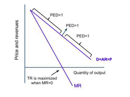
PED changes along a straight-line demand curve even though its slope is constant.
At the price-axis intercept
- quantity is close to zero;
- a small absolute quantity change is a very large percentage change;
- PED approaches infinity;
- demand is highly elastic.
Upper section
|PED| > 1
Demand is elastic.
Midpoint
|PED| = 1
Demand is unit elastic.
Lower section
|PED| < 1
Demand is inelastic.
At the quantity-axis intercept
- price is zero;
- the percentage price change basis approaches a limiting case;
- PED approaches zero;
- demand is perfectly inelastic at the intercept in the point-elasticity sense.
Why PED changes
For a straight-line demand curve, the absolute slope is constant, but the ratio of price to quantity changes.
Point-elasticity intuition:
PED magnitude = constant quantity response per price change × price / quantity
As the economy moves down the curve:
- price falls;
- quantity rises;
- price divided by quantity falls;
- PED magnitude falls.
Critical exam trap
Do not say:
A straight demand curve has constant PED.
It has constant slope, not constant elasticity.
A rectangular hyperbola demand curve, not a straight line, has unit elasticity at every point.
6. Factors affecting PED
6.1 Availability and closeness of substitutes
More and closer substitutes make demand more elastic.
Chain:
- Price rises
- consumers can switch easily
- large percentage fall in quantity demanded
- higher PED magnitude.
Examples:
- one brand of bottled water: relatively elastic because many brands exist;
- water as a broad category: more inelastic because fewer substitutes exist.
6.2 Necessity or luxury
Necessities tend to have more inelastic demand.
Luxuries tend to have more elastic demand.
The classification depends on the consumer and context.
6.3 Proportion of income spent
Products taking a large share of income tend to have more elastic demand because price changes matter more to household budgets.
A small-price everyday item may be more inelastic.
6.4 Time period
Demand often becomes more elastic over time because consumers can:
- discover substitutes;
- change habits;
- replace durable goods;
- relocate;
- alter technology.
Example:
Petrol demand may be inelastic immediately but more elastic after households can change car, transport or residence.
6.5 Breadth of market definition
Narrowly defined products usually have more substitutes and more elastic demand.
- a specific cereal brand: relatively elastic;
- breakfast food: less elastic;
- food: highly inelastic.
6.6 Habit and addiction
Habit-forming products may have more inelastic demand, particularly in the short run.
6.7 Durability and ability to postpone purchase
Demand for durable products may be elastic because consumers can delay replacement when price rises.
6.8 Brand loyalty and differentiation
Strong brand loyalty may reduce switching and make demand less elastic.
6.9 Number of uses
A price fall may create additional uses for a product, making quantity demanded more responsive.
Evaluation
No determinant acts alone. PED varies by:
- price range;
- consumer group;
- location;
- time period;
- market definition;
- availability of information.
7. PED and total expenditure
Total expenditure
Total expenditure = price × quantity demanded
For sellers, this equals total revenue from the product before considering costs.
Elastic demand
If |PED| > 1, quantity changes proportionately more than price.
- price falls
- total expenditure rises
- price rises
- total expenditure falls.
Example:
Price falls 10% and quantity demanded rises 25%. The quantity effect dominates, so expenditure rises.
Inelastic demand
If |PED| < 1, quantity changes proportionately less than price.
- price falls
- total expenditure falls
- price rises
- total expenditure rises.
Unit elastic demand
If |PED| = 1:
- the percentage price change and percentage quantity change offset;
- total expenditure remains unchanged.
Summary table
| PED | Price rises | Price falls |
|---|---|---|
| elastic | expenditure falls | expenditure rises |
| unit elastic | unchanged | unchanged |
| inelastic | expenditure rises | expenditure falls |
Straight-line demand and expenditure
Along a straight-line demand curve:
- upper elastic section: lowering price raises expenditure;
- midpoint: expenditure is maximised;
- lower inelastic section: lowering price reduces expenditure.
Important qualification
A firm normally cares about profit, not revenue alone.
A revenue-increasing price change may still reduce profit if:
- extra output has high marginal cost;
- capacity is constrained;
- quality falls;
- competitors respond.
8. Income elasticity of demand (YED)
Definition
Income elasticity of demand measures the responsiveness of quantity demanded to a change in consumer income, ceteris paribus.
Formula
YED = percentage change in quantity demanded / percentage change in income
Sign
The sign identifies whether the good is normal or inferior.
Positive YED
Quantity demanded and income move in the same direction. The product is a normal good.
Negative YED
Quantity demanded and income move in opposite directions. The product is an inferior good over the relevant income range.
Magnitude for normal goods
Income-inelastic normal good
0 < YED < 1
Quantity demanded rises less than proportionately with income. Often associated with necessities.
Unit income elasticity
YED = 1
Quantity demanded changes in the same proportion as income.
Income-elastic normal good
YED > 1
Quantity demanded rises more than proportionately with income. Often associated with luxuries.
YED calculation example
Income rises from $40 000 to $44 000. Quantity demanded rises from 200 to 230.
Percentage income change:
4 000 / 40 000 × 100 = 10%
Percentage quantity change:
30 / 200 × 100 = 15%
YED:
15% / 10% = +1.5
The product is a normal good with income-elastic demand, commonly interpreted as a luxury over this income range.
Inferior-good example
Income rises 10%, while demand for low-quality instant meals falls 5%.
YED = −5% / 10% = −0.5
The product is inferior over this range.
Critical qualification
A good is not permanently normal or inferior for every consumer and every income level.
As income rises:
- a product may first be a luxury;
- later become a necessity;
- eventually become inferior as consumers switch to higher-quality alternatives.
9. Factors affecting YED
9.1 Nature of the good
- necessities: usually positive but below 1;
- luxuries: usually above 1;
- inferior goods: negative.
9.2 Initial income level
The same product may have different YED values for low- and high-income households.
9.3 Saturation
Demand may become less income-responsive once households already own or consume large quantities.
9.4 Time period
Consumers may need time to adjust spending patterns after income changes.
9.5 Consumer preferences and demographics
Age, household size, culture and tastes affect the response.
9.6 Quality range and substitutes
Consumers may switch between lower- and higher-quality versions as income changes.
10. Business and government uses of YED
Demand forecasting
Expected economic growth raises incomes. Firms can use YED to forecast demand.
Example:
If income is expected to rise 4% and YED is +2:
expected demand increase = 8%, ceteris paribus.
Product portfolio
A firm may balance:
- luxury goods with high positive YED;
- necessities with stable demand;
- inferior goods that may perform differently in recessions.
Capacity and location
Income growth can influence investment, staffing and stock decisions.
Macroeconomic cycle
- high-YED goods may grow quickly in expansions but fall sharply in recessions;
- necessities may provide more stable revenue;
- some inferior goods may gain demand during downturns.
Government forecasting
YED can help predict demand for:
- transport;
- healthcare;
- energy;
- housing;
- public services.
11. Cross elasticity of demand (XED)
Definition
Cross elasticity of demand measures the responsiveness of quantity demanded for one product to a change in the price of another product, ceteris paribus.
Formula
XED of demand for A with respect to price of B = percentage change in quantity demanded of A / percentage change in price of B
The order matters.
The numerator is the quantity demanded of the product being studied. The denominator is the price of the related product that changes.
Positive XED: substitutes
If the price of B rises and demand for A rises, the products are substitutes.
Examples:
- tea and coffee;
- bus and train travel on the same route;
- competing phone brands.
Larger positive coefficients generally suggest closer substitutes.
Negative XED: complements
If the price of B rises and demand for A falls, the products are complements.
Examples:
- cars and petrol;
- printers and ink cartridges;
- games consoles and compatible games.
A larger negative magnitude generally suggests a stronger complementary relationship.
XED near zero: unrelated goods
A change in the price of one product has little effect on demand for the other.
Example:
- toothpaste and cinema tickets.
XED calculation example: substitutes
The price of coffee rises 20%. Demand for tea rises 10%.
XED = +10% / +20% = +0.5
Tea and coffee are substitutes.
XED calculation example: complements
The price of printers falls 10%. Demand for ink cartridges rises 25%.
XED = +25% / −10% = −2.5
Printers and cartridges are complements.
12. Factors affecting XED
12.1 Closeness of the relationship
Closer substitutes have larger positive XED values. Stronger complements have larger negative magnitudes.
12.2 Market definition
Two specific brands may be close substitutes, while broad product categories may be less substitutable.
12.3 Consumer switching costs
Contracts, compatibility and habit may weaken the response.
12.4 Time
Consumers may become more responsive as they discover alternatives or replace equipment.
12.5 Relative importance of the related product
A small change in the price of a minor complementary item may have little effect.
12.6 Compatibility and joint use
Products designed to work together may have strongly negative XED.
12.7 Brand loyalty and differentiation
Strong differentiation can reduce substitutability.
13. Business and government uses of XED
Competitive pricing
A firm can estimate how a competitor's price change affects its own demand.
Market definition
Large positive XED values may indicate that products compete in the same market.
Complementary pricing
A firm selling complementary products can coordinate prices.
Example:
- lower console price may raise demand for games;
- lower printer price may raise cartridge demand.
Mergers and competition policy
XED may provide evidence about competitive relationships, although it should not be used alone.
Product development
Businesses can identify:
- substitute threats;
- complementary opportunities;
- bundling possibilities.
14. Comparing PED, YED and XED
| Elasticity | Change causing response | Response measured | Sign mainly tells us |
|---|---|---|---|
| PED | product's own price | quantity demanded of same product | inverse price-demand relationship |
| YED | consumer income | quantity demanded | normal or inferior good |
| XED | price of another product | quantity demanded of studied product | substitutes or complements |
Formula-selection method
Ask:
- What changed?
- Whose quantity demanded changed?
- Is the changed variable own price, income or another product's price?
15. Decision-making with elasticity
Firms
PED helps with:
- price changes;
- total-revenue forecasting;
- discount strategy;
- market segmentation;
- estimating market power.
YED helps with:
- demand forecasts during growth or recession;
- capacity planning;
- product portfolio decisions;
- targeting income groups.
XED helps with:
- competitor analysis;
- complementary product strategy;
- market definition;
- response to rival price changes.
Governments
Elasticity evidence can inform:
- indirect taxation;
- transport fares;
- subsidies;
- demand forecasts;
- regulation;
- public-service capacity.
Households
Elasticity helps explain how spending patterns change when:
- prices rise;
- income changes;
- substitute prices change.
16. Limitations of elasticity estimates
Elasticity is useful, but not perfectly stable.
Ceteris paribus may fail
Other determinants may change at the same time.
Estimates depend on time period
Short-run and long-run coefficients may differ.
Market definition matters
Brand-level demand is often more elastic than category-level demand.
Data may be inaccurate
Sales data may not capture:
- informal markets;
- quality change;
- stockpiling;
- promotions;
- consumer expectations.
Coefficients may vary along a curve
A single estimate may be an average over a specific range.
Past estimates may not predict the future
Technology, tastes and competitors change.
Causation can be difficult
A price change may occur because demand changed, complicating estimation.
Profit is not revenue
A pricing decision based only on PED ignores costs.
Strong evaluation chain
Elasticity provides a structured estimate of responsiveness, but a decision should also use cost information, competitor behaviour, capacity, time period and the reliability of the underlying data.
17. Common examination traps
- Using absolute changes instead of percentage changes.
- Forgetting that PED is normally negative.
- Classifying PED using the negative sign rather than its absolute magnitude.
- Forgetting the sign of YED identifies normal versus inferior goods.
- Saying all positive-YED goods are luxuries.
- Saying all necessities have YED equal to zero.
- Reversing the numerator and denominator in XED.
- Saying a negative XED indicates substitutes.
- Saying a straight-line demand curve has constant PED.
- Confusing slope with elasticity.
- Reversing the PED-total-expenditure relationship.
- Assuming a price rise raises revenue for every product.
- Treating elasticity as fixed across all prices and time periods.
- Ignoring the market definition.
- Using PED alone to infer profit.
- Treating an inferior good as necessarily poor quality.
- Forgetting that the same good may have different YED for different incomes.
- Calling unrelated goods complements because XED is small.
18. Paper 1 technique
Calculation sequence
- Identify the correct formula.
- Calculate the percentage change in the numerator.
- Calculate the percentage change in the denominator.
- Divide.
- retain the sign;
- interpret sign and magnitude in words.
PED interpretation
- use magnitude for elastic/inelastic classification;
- explain the relative percentage response.
YED interpretation
- sign
- normal or inferior
- magnitude
- necessity-like or luxury-like responsiveness for normal goods.
XED interpretation
- positive
- substitutes
- negative
- complements
- magnitude
- closeness of relationship.
19. Paper 2 technique
Model 4-mark PED explanation
PED measures the responsiveness of quantity demanded to a change in the product's own price. It is calculated as the percentage change in quantity demanded divided by the percentage change in price. A coefficient with an absolute value greater than one indicates elastic demand because quantity demanded changes proportionately more than price.
Model 8-mark YED answer
Question:
With the help of a formula, explain YED and consider whether demand always rises at the same rate as income.
Answer structure:
- correct formula;
- responsiveness definition;
- positive YED normal good;
- negative YED inferior good;
- 0–1 necessity;
- above 1 luxury;
- YED can change with income and time;
- conclude demand need not rise at the same rate.
Model 12-mark application
Question:
Assess whether PED is sufficient for a firm deciding whether to reduce price.
Analysis:
- elastic demand
- price reduction raises revenue
- inelastic demand
- price reduction lowers revenue
- competitor reaction and substitutes affect PED;
- time period matters.
Evaluation:
- revenue is not profit;
- costs and capacity matter;
- coefficient may be estimated inaccurately;
- PED varies by price range and consumer group;
- final judgement depends on objective and context.
20. Active recall
- Define PED.
- Write the PED formula.
- Why is PED normally negative?
- How is PED classified using magnitude?
- Define perfectly elastic demand.
- Define perfectly inelastic demand.
- Why does PED vary along a straight-line curve?
- Where is PED unit elastic on a straight-line curve?
- State five determinants of PED.
- Explain the time-period effect on PED.
- State the relationship between PED and total expenditure.
- Define YED.
- What does positive YED show?
- What does negative YED show?
- Distinguish a necessity and luxury using YED.
- State four determinants of YED.
- Define XED.
- What does positive XED show?
- What does negative XED show?
- How does magnitude help interpret XED?
- Give two business uses of PED.
- Give two business uses of YED.
- Give two business uses of XED.
- State three limitations of elasticity estimates.
- Why must profit and revenue be distinguished?
21. One-minute revision
PED
% change in Qd / % change in own price
Normally negative, use magnitude to classify.
- |PED| > 1: elastic;
- |PED| = 1: unit elastic;
- |PED| < 1: inelastic.
PED and expenditure
- elastic: price and expenditure move in opposite directions;
- inelastic: price and expenditure move in the same direction;
- unit elastic: expenditure unchanged.
YED
% change in Qd / % change in income
- positive: normal;
- between 0 and 1: necessity-type normal good;
- above 1: luxury-type normal good;
- negative: inferior.
XED
% change in Qd of A / % change in price of B
- positive: substitutes;
- negative: complements;
- near zero: unrelated.
Check you have it
Question 1
Over the last ten years the price elasticity of demand for tea in many countries has risen. What is the most likely cause of this change in price elasticity?
Answer: D.
Question 2
The producer of a good with a price-elastic demand observes that a rise in its price is accompanied by a rise in total revenue. What might explain this?
Answer: B.
Question 3
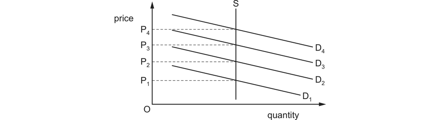
A government provides a subsidy for a product with a perfectly price inelastic demand.
What prevents producers from benefiting from this subsidy?
Answer: B.
Perfectly price inelastic demand means a vertical demand curve, consumers buy the same quantity whatever the price, so PED is zero. When the subsidy shifts the supply curve to the right, quantity cannot increase, because demand fixes it. The entire adjustment therefore falls on price, which drops by the full amount of the subsidy per unit. Producers receive the lower market price plus the subsidy, which leaves them exactly where they started: the whole benefit passes to consumers in the form of the price cut.
This mirrors the rule for taxes. The side of the market that is less responsive to price captures the benefit of a subsidy and bears the burden of a tax, and demand here is completely unresponsive.
Why the other options are wrong:
- A says price elasticity of demand is infinite, which describes perfectly elastic demand, a horizontal curve. That is the opposite case, and it is the one where producers keep the whole subsidy.
- C describes demand as relatively elastic, contradicting the premise.
- D correctly calls demand inelastic but claims the price reduction is small. With PED of zero the price fall is as large as it can possibly be, because price is the only variable free to move.
Critical final rule
Calculate, retain the sign, interpret the magnitude, then apply it to the decision.
What the syllabus asks for on this topicOfficial syllabus coverage · Product mastery map
Official syllabus coverage
Students must understand:
- 2.2.1 definitions of price elasticity, income elasticity and cross elasticity of demand: PED, YED and XED;
- 2.2.2 formulae and calculations for PED, YED and XED;
- 2.2.3 the significance of relative percentage changes and the size and sign of each coefficient;
- 2.2.4 perfectly elastic, elastic, unitary elastic, inelastic and perfectly inelastic demand;
- 2.2.5 variation in PED along a straight-line demand curve;
- 2.2.6 factors affecting PED, YED and XED;
- 2.2.7 the relationship between PED and total expenditure;
- 2.2.8 implications of PED, YED and XED for decision-making.
Product mastery map
The portal tracks ten separate skills:
- define PED, YED and XED;
- calculate percentage changes and elasticity coefficients;
- interpret coefficient signs and magnitudes;
- classify PED values and extreme cases;
- explain changing PED along a straight-line demand curve;
- analyse determinants of PED;
- analyse determinants of YED;
- analyse determinants of XED;
- apply PED to total expenditure and revenue;
- use elasticity evidence in business and government decisions.
Related CIE 9708 topics
Not the topic you were looking for? Describe what you are stuck on in your own words and we will take you to the notes that answer it.