Costs, Revenue and Profit
Types of Cost, Revenue and Profit, Short-run and Long-run Production
Contents: 17 sections
1. Why this topic matters
A firm turns inputs into output, incurs costs, earns revenue and may make profit or loss. Topic 7.5 builds the analytical toolkit needed for every later theory-of-the-firm topic. It explains:
- how output changes when a variable factor is added to fixed factors;
- how short-run product relationships generate short-run cost curves;
- how changing the scale of all inputs affects long-run production and costs;
- why economies and diseconomies of scale matter;
- how to calculate total, average and marginal revenue; and
- how economists define and calculate normal, supernormal and subnormal profit.
The most important discipline is to keep distinct ideas separate:
- short run versus long run is about whether factors can be varied;
- diminishing returns is a short-run production concept;
- returns to scale is a long-run physical-output concept;
- economies of scale is a long-run average-cost concept;
- revenue is not profit; and
- normal profit is not zero accounting profit.
2. Short run and long run
2.1 The short run
The short run is a period in which at least one factor of production is fixed. A fixed factor cannot be changed within the relevant decision period. Other factors are variable.
A restaurant may be able to vary staff hours and ingredients this week but be unable to change the size of its premises. For that decision, labour and ingredients are variable while the building is fixed.
There is no universal number of months that defines the short run. The relevant period differs across industries. A street-food stall may change most inputs quickly; a railway or semiconductor plant may require years to alter capacity.
2.2 Fixed and variable factors
A fixed factor does not change as output changes in the short run. A variable factor can change as output changes.
The classification concerns the quantity of the input, not whether a bill is paid regularly. A monthly electricity standing charge may be fixed, while electricity used by each machine may be variable.
2.3 The long run
The long run is a period in which all factors of production are variable. The firm can change plant size, machinery, land, organisational structure and labour.
Long run does not mean that every firm necessarily expands. It means that no factor is fixed. A firm may expand, contract, adopt a different production method or leave the industry.
3. The short-run production function
A production function shows the maximum output obtainable from different combinations of inputs with existing technology.
In the short run, at least one input is fixed. The standard model varies one factor, often labour, while capital is fixed.
3.1 Total product
Total product (TP) is the total output produced by a given quantity of a variable factor.
3.2 Average product
Average product (AP) is output per unit of the variable factor:
AP = TP / units of variable factor
If 6 workers produce 90 units, AP = 90 / 6 = 15 units per worker.
3.3 Marginal product
Marginal product (MP) is the change in total product caused by an additional unit of the variable factor:
MP = change in TP / change in variable factor
When labour rises in whole workers, MP is often the increase in TP from employing the next worker.
3.4 Worked product table
| Workers | TP | MP | AP |
|---|---|---|---|
| 0 | 0 | – | – |
| 1 | 12 | 12 | 12.0 |
| 2 | 28 | 16 | 14.0 |
| 3 | 48 | 20 | 16.0 |
| 4 | 64 | 16 | 16.0 |
| 5 | 75 | 11 | 15.0 |
| 6 | 81 | 6 | 13.5 |
| 7 | 84 | 3 | 12.0 |
| 8 | 84 | 0 | 10.5 |
Key observations:
- TP rises while MP is positive.
- TP is maximised when MP becomes zero.
- TP falls if MP becomes negative.
- AP rises when MP is above AP.
- AP falls when MP is below AP.
- MP crosses AP at AP's maximum in a smooth-curve model.
The average–marginal rule is general: a marginal value above the average pulls the average up; a marginal value below the average pulls it down.
4. The law of diminishing returns
The law of diminishing returns, also called the law of variable proportions, states that when additional units of a variable factor are combined with fixed factors, marginal product will eventually fall, other things equal.
4.1 Why it happens
Initially, extra workers may permit specialisation and fuller use of fixed capital, so MP can rise. Eventually the fixed input becomes a constraint. Workers may wait for machinery, crowd the workspace or duplicate tasks. Each additional worker then adds less output than the previous one.
4.2 When diminishing returns begin
Diminishing marginal returns begin when MP starts to fall, not when:
- TP begins to fall;
- MP becomes negative;
- AP begins to fall; or
- costs begin to rise in total.
In the worked table, MP peaks at 20 with the third worker and falls to 16 with the fourth. Diminishing returns therefore begin with the fourth worker, even though TP continues to rise.
4.3 Conditions for the law
The analysis assumes:
- at least one factor is fixed;
- units of the variable factor are sufficiently comparable;
- technology and input quality are unchanged; and
- the production process is otherwise unchanged.
Diminishing returns does not mean that workers become less skilled. It describes the marginal output generated when more variable input is combined with limited fixed input.
5. The short-run cost function
5.1 Fixed costs and variable costs
Fixed costs (FC) do not vary with output in the short run. Examples may include rent for existing premises, insurance and a fixed licence fee.
Variable costs (VC) vary with output. Examples may include raw materials, hourly production labour, packaging and usage-related energy.
A cost is not fixed merely because it is paid monthly, nor variable merely because its market price can change. The question is whether total spending on it changes as the firm's output changes in the relevant short run.
5.2 Total costs
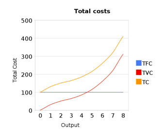
- Total fixed cost (TFC) = total fixed costs.
- Total variable cost (TVC) = total variable costs.
- Total cost (TC) = TFC + TVC.
At zero output, TVC is normally zero, but TFC remains, so TC = TFC.
5.3 Average costs
- Average fixed cost (AFC) = TFC / Q
- Average variable cost (AVC) = TVC / Q
- Average total cost (ATC or AC) = TC / Q
Because TC = TFC + TVC:
ATC = AFC + AVC
5.4 Marginal cost
Marginal cost (MC) is the change in total cost caused by producing an additional unit:
MC = change in TC / change in Q
Since fixed cost does not change with output:
MC = change in TVC / change in Q
MC is not TC divided by output. That is average total cost.
5.5 Worked cost calculation
Suppose Q = 10, TFC = 120 and TVC = 180.
- TC = 120 + 180 = 300
- AFC = 120 / 10 = 12
- AVC = 180 / 10 = 18
- ATC = 300 / 10 = 30
If TC rises from 300 at Q = 10 to 326 at Q = 11:
- MC of the eleventh unit = 326 − 300 = 26.
6. Shapes of short-run cost curves
6.1 Total fixed, variable and total cost
- TFC is horizontal when plotted against output because it does not change.
- TVC usually rises as output rises.
- TC lies vertically above TVC by the constant amount TFC.
- TC and TVC therefore have the same slope at each output.
6.2 Average fixed cost
AFC continually falls as output rises because the same TFC is spread across more units. It approaches zero but does not become zero while TFC is positive.
6.3 AVC and ATC
AVC and ATC are conventionally U-shaped in the short-run model.
- At low output, increasing marginal returns and specialisation may reduce per-unit variable cost.
- Once diminishing returns become sufficiently strong, additional output requires increasingly large additions of variable input, raising AVC and ATC.
The vertical distance between ATC and AVC equals AFC, so it narrows as output increases.
6.4 MC and the average curves
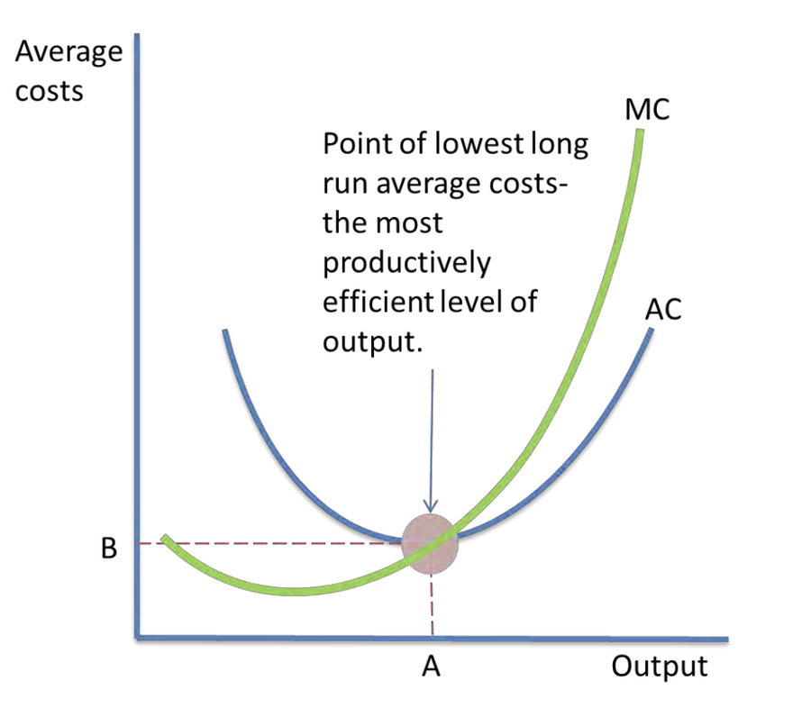
MC cuts AVC and ATC at their minimum points.
- When MC is below an average, it pulls that average down.
- When MC is above an average, it pulls that average up.
MC may start rising before AVC and ATC reach their minimum values. A rising marginal value can still be below the average and continue to pull the average down.
6.5 Cost-curve shifts
A change in a fixed cost, such as rent on existing premises:
- shifts TFC and TC;
- shifts AFC and ATC;
- does not directly shift TVC, AVC or MC.
A change in a variable input price, such as the hourly wage or material cost:
- shifts TVC and TC;
- shifts AVC, ATC and MC;
- does not shift TFC or AFC.
7. Connecting product curves to cost curves
Under the simplifying assumptions that labour is the only variable factor and the wage per worker is constant:
MC = wage / MP
AVC = wage / AP
Therefore:
- when MP rises, MC falls;
- when MP falls, MC rises;
- when AP rises, AVC falls;
- when AP falls, AVC rises;
- maximum MP corresponds to minimum MC; and
- maximum AP corresponds to minimum AVC.
This inverse relationship explains why diminishing marginal returns eventually create rising marginal cost.
These formulas depend on the stated assumptions. If several variable inputs change or factor prices vary, the relationship is more complex.
A further correction is important: the worker level that maximises AP does not automatically maximise profit or minimise total cost for a chosen output. A firm's optimal employment decision depends on the value of marginal output and the cost of the factor, which is developed further in labour-market analysis.
8. The long-run production function and returns to scale
In the long run, all factors are variable. The firm can change the scale of the whole operation.
Returns to scale compare the proportional change in output with an equal proportional change in all inputs.
8.1 Increasing returns to scale
If all inputs rise by a given proportion and output rises by a larger proportion, there are increasing returns to scale.
Example: all inputs double and output rises by 140%.
8.2 Constant returns to scale
If all inputs rise by a given proportion and output rises by the same proportion, there are constant returns to scale.
Example: all inputs double and output doubles.
8.3 Decreasing returns to scale
If all inputs rise by a given proportion and output rises by a smaller proportion, there are decreasing returns to scale.
Example: all inputs double but output rises by only 70%.
8.4 Returns to scale versus diminishing returns
Do not confuse the two:
- diminishing returns: short run, one variable factor added to fixed factors;
- returns to scale: long run, all inputs change proportionately.
Returns to scale is a physical production relationship. Economies of scale concerns average cost and may also reflect purchasing, financing or organisational advantages.
9. Long-run costs, LRAC and minimum efficient scale
9.1 The long-run average cost curve
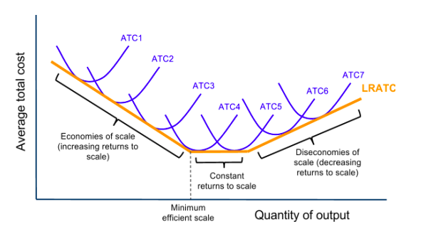
Long-run average cost (LRAC) shows the lowest attainable average cost of producing each output when all inputs and plant size can be varied.
It is often described as a planning curve or an envelope of possible short-run average cost (SRAC) curves. For each output, the firm chooses the plant and input combination with the lowest available average cost.
LRAC is commonly drawn falling, then flat or gently curved, then rising:
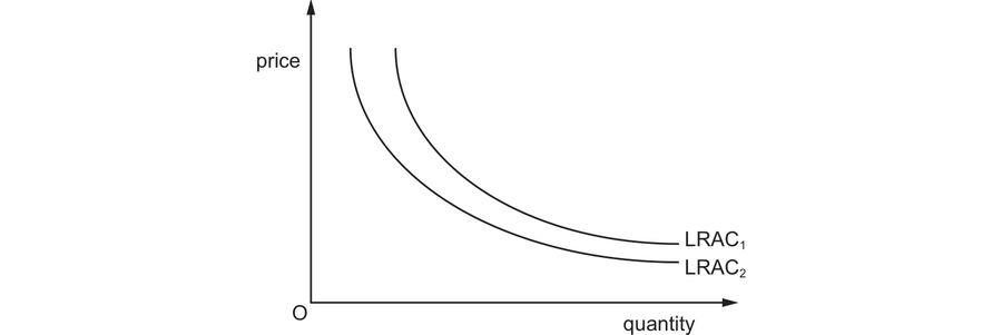
- falling LRAC reflects economies of scale;
- a flat minimum range reflects broadly constant average costs; and
- rising LRAC reflects diseconomies of scale.
Real LRAC curves need not be perfectly smooth or strongly U-shaped. The diagram is a model.
9.2 Minimum efficient scale
Minimum efficient scale (MES) is the lowest level of output at which the firm reaches the minimum long-run average cost, or has captured the available economies of scale to the point that further expansion does not materially lower LRAC.
MES matters for market structure:
- a low MES relative to market demand can support many efficient firms;
- a high MES relative to market demand may support only a few large firms.
Detailed market-structure implications are developed in Topic 7.6.
10. Internal economies of scale
Internal economies of scale arise from the growth of the individual firm and lower that firm's long-run average cost.
10.1 Technical economies
Large-scale production can make specialised machinery viable, permit fuller use of indivisible equipment and support more efficient production flows.
10.2 Managerial economies
A large firm can employ specialist managers in finance, logistics, marketing, data, engineering and human resources. Specialisation can improve decisions and reduce average cost.
10.3 Purchasing economies
Bulk purchases can give the firm bargaining power or lower suppliers' delivery and administration cost per unit.
10.4 Marketing economies
Advertising, distribution systems and brand development may be spread across a larger output. Marketing expenditure does not need to rise in the same proportion as sales.
10.5 Financial economies
Larger, diversified firms may be viewed as lower-risk borrowers and may access finance at lower interest rates or issue securities more cheaply.
10.6 Risk-bearing and research economies
A larger firm may spread risk across products and markets, fund research and development, and undertake projects with high fixed costs.
Economies of scale lower average cost only if the cost saving is greater than any new cost created by expansion.
11. External economies of scale
External economies of scale arise from expansion of the industry or economic cluster and lower the costs of firms within it, including firms that have not themselves grown.
Examples include:
- a pool of specialised skilled labour;
- specialist suppliers locating nearby;
- shared logistics and digital infrastructure;
- training institutions and research networks;
- knowledge spillovers between firms; and
- improved reputation of a regional cluster.
The distinction is based on the source of the saving:
- internal economy: caused by growth of the firm;
- external economy: caused by growth or development outside the individual firm, often the industry or location.
External economies may shift the long-run cost conditions of many firms downward.
12. Diseconomies of scale
12.1 Internal diseconomies of scale
Internal diseconomies of scale arise within an expanding firm and increase its LRAC.
Possible causes include:
- longer communication chains;
- coordination problems across divisions and countries;
- slower decision-making and bureaucracy;
- weaker monitoring and loss of control;
- alienation and reduced worker motivation;
- duplication of functions; and
- integration failures after rapid expansion.
12.2 External diseconomies of scale
External diseconomies of scale arise as an industry or cluster expands and raise the costs of firms within it.
Examples include:
- higher local wages caused by competition for scarce skills;
- rising land and commercial rents;
- congestion and delivery delays;
- pressure on infrastructure;
- higher prices for specialised inputs; and
- environmental or regulatory costs generated by industry concentration.
A single firm may experience falling internal costs while external industry congestion pushes costs upward. The net LRAC effect depends on the relative strengths of these influences.
13. Revenue
13.1 Total revenue
Total revenue (TR) is the firm's receipts from sales:
TR = price × quantity sold
13.2 Average revenue
Average revenue (AR) is revenue per unit sold:
AR = TR / Q
For a firm charging one price for all units, AR equals price.
13.3 Marginal revenue
Marginal revenue (MR) is the change in TR from selling an additional unit:
MR = change in TR / change in Q
Example:
| Q | Price | TR | MR |
|---|---|---|---|
| 1 | 20 | 20 | 20 |
| 2 | 18 | 36 | 16 |
| 3 | 16 | 48 | 12 |
| 4 | 14 | 56 | 8 |
| 5 | 12 | 60 | 4 |
| 6 | 10 | 60 | 0 |
| 7 | 8 | 56 | −4 |
TR rises when MR is positive, is maximised when MR is zero in a smooth model, and falls when MR is negative.
For a price-taking firm, price, AR and MR are equal. For a firm facing a downward-sloping demand curve, reducing price to sell more may make MR lower than AR. Detailed market-structure applications belong to Topic 7.6.
14. Normal, supernormal and subnormal profit
14.1 Economic cost and normal profit
Economists include opportunity cost in total cost. The entrepreneur's normal profit is the minimum return required to keep enterprise and capital in their current use. It is therefore part of economic cost.
14.2 Normal profit
A firm earns normal profit when:
TR = total economic cost
The firm's economic profit is zero, but the owner still receives the normal return included in cost.
14.3 Supernormal profit
Supernormal profit exists when:
TR > total economic cost
It is the return above normal profit, also called abnormal or economic profit.
14.4 Subnormal profit
Subnormal profit exists when:
TR < total economic cost
It is an economic loss. The firm earns less than the normal return required to keep all resources in their present use.
Subnormal profit does not necessarily mean negative accounting profit. A firm may cover explicit accounting costs but fail to cover the opportunity cost of owner-supplied capital and enterprise.
14.5 Profit calculations
Total economic profit = TR − TC
At a given output:
profit per unit = AR − AC
Therefore:
total profit = (AR − AC) × Q
Worked example: supernormal profit
A firm sells 500 units at $18. Its ATC is $14.
- TR = 18 × 500 = $9,000
- TC = 14 × 500 = $7,000
- supernormal profit = $2,000
Worked example: subnormal profit
A firm sells 300 units at $25. Its ATC is $29.
- TR = 25 × 300 = $7,500
- TC = 29 × 300 = $8,700
- economic profit = −$1,200
- subnormal profit/economic loss = $1,200
A loss rectangle on a graph has height AC − AR and width Q. A supernormal-profit rectangle has height AR − AC and width Q.
15. Integrated analysis and common traps
15.1 A complete production-to-cost chain
More variable input with fixed capital → MP may initially rise → MC falls → diminishing returns begin → MP falls → MC rises → eventually AP falls → AVC rises.
15.2 A complete scale chain
All inputs expand → specialisation/indivisibilities/purchasing advantages → output or cost efficiency improves → LRAC falls → MES reached → further coordination problems may eventually raise LRAC.
15.3 Common examination errors
- Defining short run as a fixed calendar period.
- Saying diminishing returns begin when MP is negative.
- Calculating MP as TP divided by labour.
- Calculating MC as TC divided by output.
- Treating monthly payment as proof that a cost is fixed.
- Saying a rise in fixed cost shifts MC.
- Confusing diminishing returns with decreasing returns to scale.
- Treating returns to scale and economies of scale as exact synonyms.
- Defining MES as the output where short-run AC is lowest without reference to LRAC.
- Calling all industry growth benefits internal economies.
- Treating TR as profit.
- Describing normal profit as no reward to the entrepreneur.
- Reporting a negative number without identifying it as subnormal profit/economic loss.
- Importing market-structure conclusions before analysing costs and revenues accurately.
16. Paper 3 and Paper 4 mastery
For calculations:
- write the formula;
- substitute values carefully;
- preserve units;
- show changes between rows for marginal values; and
- interpret the result economically.
For diagrams:
- label both axes;
- identify TP/AP/MP or AFC/AVC/ATC/MC clearly;
- mark the relevant maxima or minima;
- explain relationships rather than relying on curve shape alone; and
- distinguish short-run from long-run diagrams.
For essays, build chains and then evaluate conditions. For example, an economy of scale lowers LRAC only when the saving is realised and is not outweighed by coordination problems. A high MES may encourage concentration, but market demand, entry conditions and technology also matter.
Check you have it
Question 1
The diagram shows a firm in imperfect competition. It changed its aim from profit maximising to sales revenue maximising. Which type of profit was it making in each case?
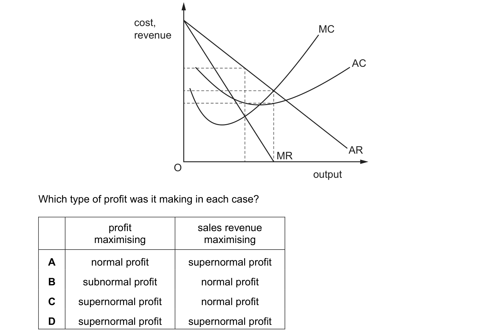
Answer: D.
Question 2
The diagram shows the short-run equilibrium for a firm operating in a monopolistically competitive market. What is not likely to occur at the long-run equilibrium?
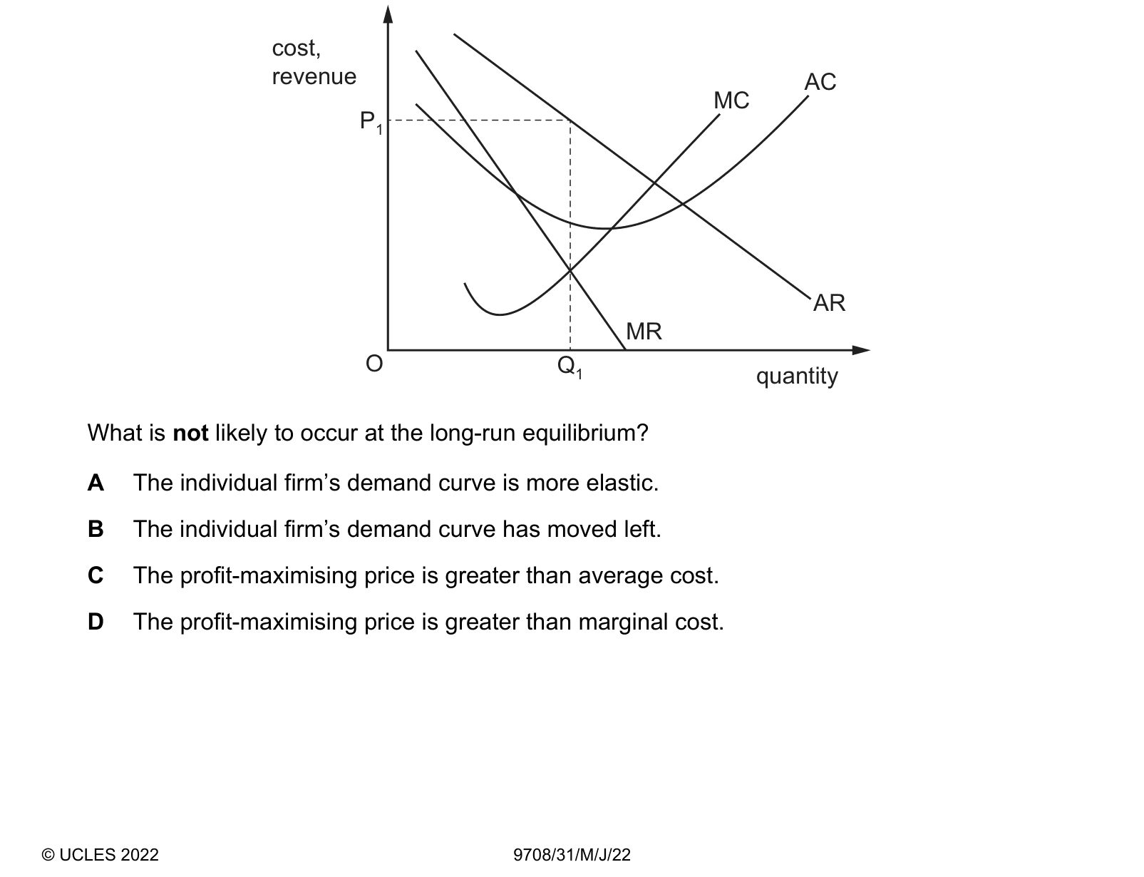
Answer: C.
Question 3
The diagram shows the cost and revenue curves of a profit-maximising monopolist. What measures the total monopoly profit made by the firm?
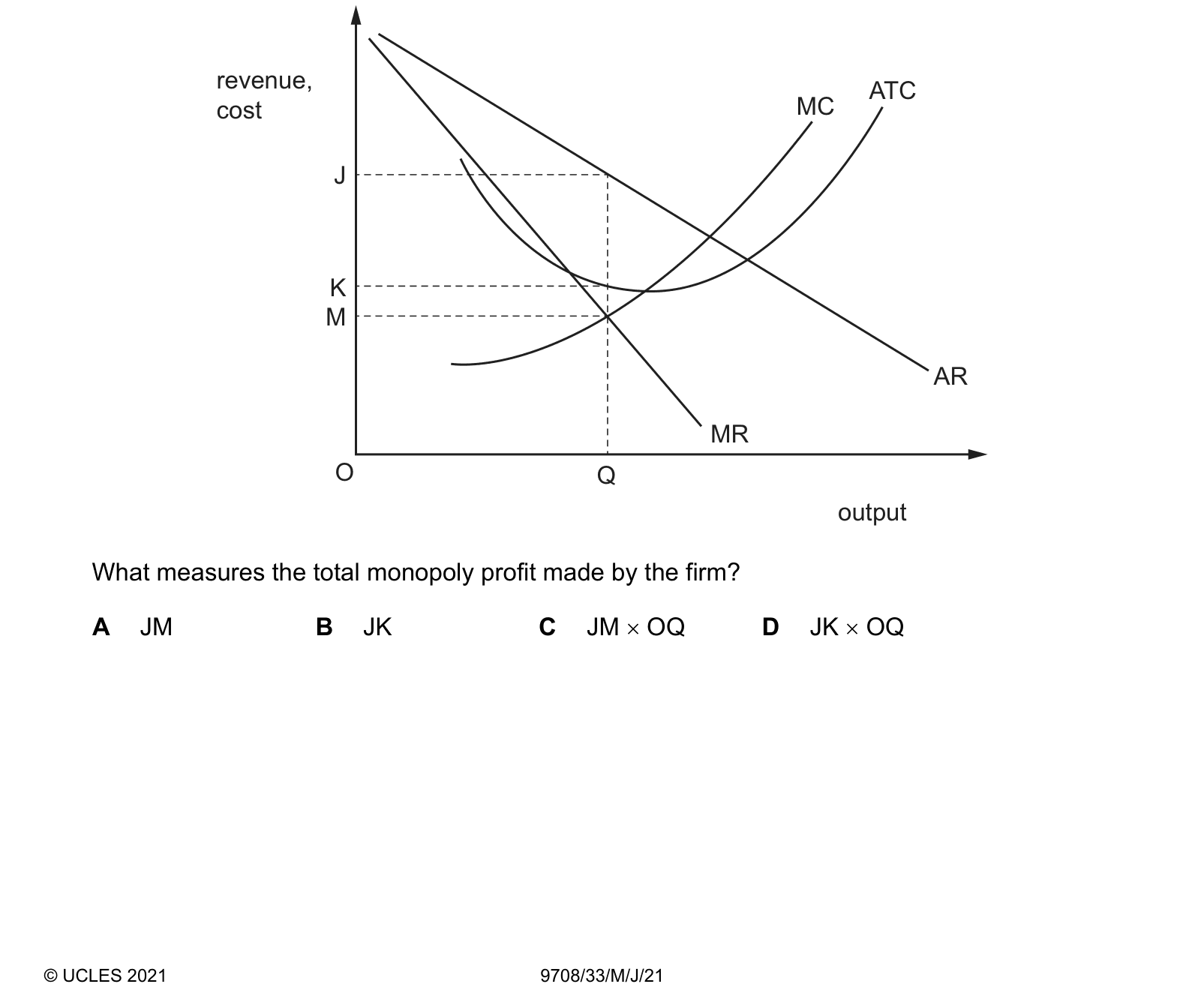
Answer: D.
17. Final checklist
A fully prepared learner can:
- distinguish short and long run using fixed and variable factors;
- calculate and interpret TP, AP and MP;
- locate the start of diminishing returns;
- calculate every required short-run cost measure;
- explain all standard short-run cost-curve relationships;
- connect product and cost curves under stated assumptions;
- identify increasing, constant and decreasing returns to scale;
- explain LRAC and MES;
- classify internal/external economies and diseconomies;
- calculate TR, AR and MR;
- define normal, supernormal and subnormal profit; and
- calculate total and per-unit profit or loss.

Related CIE 9708 topics
Not the topic you were looking for? Describe what you are stuck on in your own words and we will take you to the notes that answer it.