Indifference Curves and Budget Lines
Contents: 11 sections
Cambridge International AS & A Level Economics 9708 (A Level) Current syllabus: 2026–2028, Version 2 Official syllabus points: 7.2.1–7.2.4
Exam Essentials
1. What is an indifference curve?
An indifference curve shows all combinations of two goods that give a consumer the same level of satisfaction or utility.
If bundle A and bundle B lie on the same indifference curve, the consumer is assumed to be indifferent between them. This does not mean that the bundles contain the same quantities. It means that the consumer regards the gains from having more of one good as exactly compensating for having less of the other.
A simple bundle table
Suppose a consumer regards the following combinations as equally satisfactory:
| Bundle | Units of X | Units of Y |
|---|---|---|
| A | 1 | 12 |
| B | 2 | 8 |
| C | 4 | 5 |
| D | 7 | 3 |
Plotting these bundles and joining them produces an indifference curve.
Core properties of standard indifference curves
Under the usual assumptions, indifference curves are:
- downward sloping: to keep utility unchanged, gaining more of X normally requires giving up some Y;
- convex to the origin: the marginal rate of substitution usually diminishes as the consumer moves down the curve;
- non-intersecting: two curves cannot cross if preferences are consistent;
- ranked: a curve farther from the origin normally represents a higher level of utility when both goods are desirable;
- thin rather than thick: a thick band would contain distinct bundles that could not all represent exactly the same utility level.
These properties are consequences of assumptions, not physical laws. Perfect substitutes may generate straight-line indifference curves. Perfect complements may generate right-angled curves. A good and a bad may create an upward-sloping curve. Cambridge questions usually use the standard case of two desirable goods unless the context says otherwise.
2. Marginal rate of substitution
The marginal rate of substitution of X for Y (MRSxy) is the quantity of Y a consumer is willing to give up to obtain one additional unit of X while remaining on the same indifference curve.
For a movement between two discrete bundles:
MRSxy = amount of Y given up / additional amount of X obtained
The slope of an indifference curve is negative, so the MRS is often stated as an absolute value.
Example
Moving from bundle A to bundle B gives the consumer 2 extra units of X and requires giving up 6 units of Y.
MRSxy = 6 / 2 = 3
The consumer is willing to give up 3 units of Y for each additional unit of X over that movement.
Why the MRS normally diminishes
At the upper-left of a standard curve, the consumer has much Y and little X. An extra unit of X is relatively valuable, so the consumer may be willing to give up a large amount of Y.
Farther down the curve, the consumer has more X and less Y. Another unit of X is less valuable relative to scarce Y, so the amount of Y willingly sacrificed falls.
This diminishing MRS explains the convex shape of the standard indifference curve.
MRS and marginal utility
Where marginal utilities can be used, the MRS can be expressed as:
MRSxy = MUx / MUy
This creates the bridge between Topic 7.1 and Topic 7.2. The indifference-curve model does not require utility to be measured in cardinal “utils”; it only requires preferences to be ranked consistently.
The budget line
3. Meaning of a budget line
A budget line shows every combination of two goods that exactly exhausts a consumer’s income at given prices.
If income is M, the price of X is Px and the price of Y is Py:
PxX + PyY = M
The line is a constraint, not a statement of preference.
- Bundles on the line are affordable and use all income.
- Bundles inside the line are affordable but leave some income unspent.
- Bundles outside the line are unaffordable at the current income and prices.
Intercepts
If the consumer spends all income on X:
maximum X = M / Px
If the consumer spends all income on Y:
maximum Y = M / Py
Slope
With X on the horizontal axis and Y on the vertical axis:
slope of the budget line = −Px / Py
The absolute slope is the market opportunity cost of X in terms of Y. To obtain one more unit of X, the consumer must give up Px/Py units of Y.
Worked example
Income is £60. X costs £5 and Y costs £10.
5X + 10Y = 60
- X-intercept = 60/5 = 12
- Y-intercept = 60/10 = 6
- slope = −5/10 = −0.5
A bundle of 6X and 3Y costs £60 and lies on the line. A bundle of 4X and 2Y costs £40 and lies inside it. A bundle of 10X and 3Y costs £80 and lies outside it.
4. Causes of a change in the budget line
The position and slope of the budget line depend on income and prices.
A change in money income
If both prices are unchanged:
- higher income shifts the budget line outward in a parallel way;
- lower income shifts it inward in a parallel way.
The slope is unchanged because Px/Py is unchanged. Both intercepts change in the same proportion as income.
A change in the price of one good
If income and the other price are unchanged, the line pivots.
For example, if Px falls:
- the maximum affordable quantity of X rises;
- the X-intercept moves outward;
- the Y-intercept is unchanged;
- the line becomes flatter because Px/Py falls.
If Px rises, the opposite occurs.
Changes in both prices
- If both prices fall in the same proportion, the budget line shifts outward in parallel.
- If both prices rise in the same proportion, it shifts inward in parallel.
- If prices change by different proportions, the line both changes position and changes slope.
A proportional fall in both prices has the same effect on purchasing power as a proportional rise in income, although nominal income has not changed.
Taxes, subsidies and rationing
A per-unit tax on X raises its effective consumer price and pivots the line inward on the X-axis. A per-unit subsidy has the opposite effect. Quantity restrictions or block pricing can create a kinked or discontinuous budget constraint rather than one straight line. These are useful extensions but the standard Cambridge model normally begins with constant unit prices.
Consumer equilibrium
5. The highest attainable indifference curve
A rational consumer chooses the affordable bundle that lies on the highest attainable indifference curve.
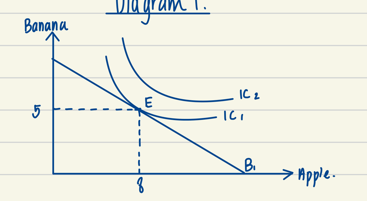
Read the diagram for what it rules out as much as what it shows. IC2 is not unreachable because the consumer does not want it, they would prefer it; it is unreachable because every point on it costs more than the income the budget line represents. And E is not merely a point the budget line happens to cross, it is the only point where the line touches IC1 rather than cutting through it, which is what tangency means.
In the standard smooth interior solution, equilibrium occurs where the budget line is tangent to an indifference curve:
MRSxy = Px / Py
Using marginal utilities:
MUx / MUy = Px / Py
which is equivalent to:
MUx/Px = MUy/Py
The condition from Topic 7.1 and the tangency condition from Topic 7.2 describe the same underlying idea: the consumer’s willingness to trade goods must match the trade-off imposed by market prices.
Why a non-tangency point is not optimal
Suppose MRSxy > Px/Py. The consumer values an extra unit of X more highly than the market cost of X in terms of Y. Moving along the budget line towards more X can reach a higher indifference curve.
If MRSxy < Px/Py, the consumer should move towards more Y.
At tangency, there is no feasible small reallocation that raises utility.
The tangency is not enough by itself
The chosen point must also:
- lie on the budget constraint;
- be on the highest attainable curve;
- satisfy the assumed shape of preferences;
- be feasible given non-negative quantities.
With perfect substitutes or very strong preferences, the optimum may be a corner solution at an intercept rather than a tangency. This is one reason not to treat the tangency rule as universal.
Income, substitution and price effects
6. The price effect
The price effect is the total change in quantity demanded caused by a change in the good’s own price, holding other determinants constant.
It can be separated into:
price effect = substitution effect + income effect
This decomposition helps explain why the demand curve normally slopes downward and why Giffen goods are theoretically possible.
7. The substitution effect
The substitution effect is the change in consumption caused by a change in relative prices, with the consumer compensated so that the original level of utility can still be achieved.
When the price of X falls, X becomes cheaper relative to Y. The consumer substitutes towards X and away from Y.
When the price of X rises, the consumer substitutes away from X.
For standard convex preferences, the substitution effect always moves quantity demanded in the opposite direction to the price change.
Showing the substitution effect on a diagram
Using the Hicksian approach:
- start at the original tangency between the original budget line and indifference curve;
- draw the new budget line after the price change;
- draw a compensated budget line parallel to the new budget line but tangent to the original indifference curve;
- movement from the original optimum to the compensated optimum is the substitution effect;
- movement from the compensated optimum to the final optimum is the income effect.
The compensated line has the new relative-price slope but adjusts purchasing power to keep utility at the original level.
8. The income effect
The income effect is the change in consumption caused by the change in real purchasing power resulting from a price change.
A fall in the price of X makes the consumer’s money income able to buy more. Real income rises. A rise in price lowers real income.
The direction of the income effect depends on whether X is normal or inferior.
Normal goods
9. Price change for a normal good
A normal good is one for which quantity demanded rises when income rises, other things equal.
Consider a fall in the price of X:
- substitution effect: X is relatively cheaper, so quantity of X rises;
- income effect: real income rises and X is normal, so quantity of X rises;
- total price effect: both effects reinforce each other, so quantity demanded rises.
For a price rise, both effects reduce quantity demanded.
| Price change for X | Substitution effect on X | Income effect for normal X | Total price effect |
|---|---|---|---|
| Price falls | Quantity rises | Quantity rises | Quantity rises strongly |
| Price rises | Quantity falls | Quantity falls | Quantity falls strongly |
This gives the usual downward-sloping demand curve.
Inferior goods
10. Price change for an inferior good
An inferior good is one for which quantity demanded falls when income rises, other things equal.
Consider a fall in the price of inferior good X:
- substitution effect: X is relatively cheaper, so quantity of X rises;
- income effect: real income rises, so the consumer buys less X because it is inferior;
- the effects move in opposite directions.
For an ordinary inferior good, the substitution effect is larger than the opposing income effect. Quantity demanded therefore still rises when price falls. Its demand curve remains downward sloping.
| Price change for X | Substitution effect on X | Income effect for inferior X | Ordinary total effect |
|---|---|---|---|
| Price falls | Quantity rises | Quantity falls | Quantity rises if substitution dominates |
| Price rises | Quantity falls | Quantity rises | Quantity falls if substitution dominates |
The key distinction is:
Inferior does not automatically mean Giffen.
Most inferior goods are not Giffen goods.
Giffen goods
11. The Giffen case
A Giffen good is an inferior good for which the income effect is sufficiently strong to outweigh the substitution effect.
Consider a rise in the price of staple good X:
- substitution effect: the consumer would normally buy less X because it is relatively more expensive;
- income effect: the price rise makes the consumer substantially poorer in real terms;
- because X is strongly inferior and absorbs a large share of the budget, the consumer may cut purchases of more expensive foods and buy more of staple X;
- if this income effect is larger than the substitution effect, quantity demanded of X rises as its price rises.
The demand curve is upward sloping over the relevant range.
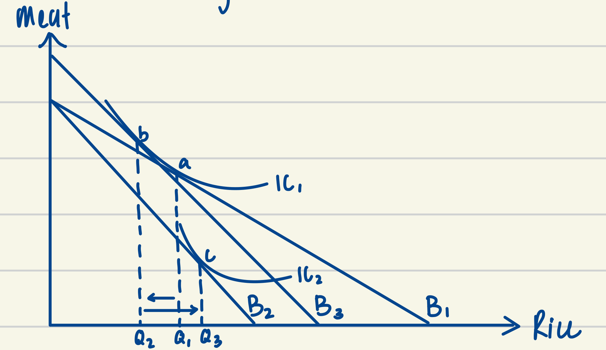
The diagram is worth reading in the order it was drawn, because the whole result is in the two arrows. a to b is the substitution effect, isolated by the compensating budget line B3: rice is now relatively dearer, so the consumer moves away from it and quantity falls from Q1 to Q2. b to c is the income effect: the price rise has made the consumer genuinely poorer, and because rice is strongly inferior they respond by buying more of it, from Q2 to Q3.
The second arrow is longer than the first. That is the entire Giffen condition drawn rather than asserted, and it is why Q3 lies to the right of Q1: the quantity demanded of rice has risen even though its price has risen. Note also that c sits on the lower curve IC2, which is the diagram insisting that the consumer is worse off, however much more rice they end up buying.
Conditions that make a Giffen outcome more plausible
A Giffen outcome is more plausible when:
- the good is strongly inferior;
- it takes a large share of a low-income consumer’s budget;
- there are few close, cheaper substitutes;
- the consumer must maintain a minimum level of calories or basic consumption;
- the real-income effect of the price change is large.
A Giffen good is not the same as a Veblen good. A Veblen good may be demanded because a higher price signals status or exclusivity; that is a preference or signalling explanation, not an income-effect explanation.
The crucial hierarchy
- All Giffen goods are inferior.
- Not all inferior goods are Giffen.
- A normal good cannot be Giffen in the standard model because its income and substitution effects reinforce each other after a price fall.
Diagram mastery
12. How to construct a price-effect diagram accurately
For a fall in the price of X, with X on the horizontal axis:
- draw the original budget line B1;
- draw the new budget line B2 pivoting outward from the unchanged Y-intercept;
- mark original equilibrium A on indifference curve I1;
- mark final equilibrium C on a new indifference curve;
- draw compensated line Bc parallel to B2 and tangent to I1 at B;
- label A → B as substitution effect;
- label B → C as income effect;
- label A → C as price effect.
For a normal good, B and C are both to the right of A after a price fall.
For an inferior good, B is to the right of A but C lies to the left of B. If C remains to the right of A, the good is ordinary inferior. If C lies to the left of A, the income effect dominates and the good is Giffen.
Frequent diagram errors
- drawing the compensated line parallel to the original rather than the new budget line;
- placing the compensated line on the new indifference curve rather than the original one;
- calling the total price effect the substitution effect;
- showing a parallel movement when only one price changes;
- changing both intercepts when one price changes;
- labelling any inferior good as Giffen;
- using a static diagram without stating whether the price rose or fell;
- confusing nominal income with real purchasing power.
Limitations of the indifference-curve model
13. Preference assumptions
The model assumes consumers can rank all bundles (completeness) and do so consistently (transitivity).
If a consumer prefers A to B and B to C, transitivity requires A to be preferred to C. Real choices can be inconsistent because of framing, context, changing moods or limited attention.
The model also assumes preferences are reasonably stable during the analysis. Advertising, social influence, habit, learning and expectations can change preferences.
14. Information and calculation
Consumers may not know all prices, qualities, future consequences or available alternatives. Comparing many bundles is costly and time-consuming. Consumers may satisfice, follow rules of thumb or copy others rather than solve a formal optimisation problem.
15. Ordinal utility is still unobservable
Indifference curves avoid the need to measure utility in cardinal units, but the curves themselves cannot normally be observed directly. Economists infer preferences from choices, and observed choices may also reflect mistakes, constraints or strategic behaviour.
16. Two-good simplification
The standard diagram places only two goods on the axes. “All other goods” can be grouped into a composite good, but this hides important interactions, complementarities and changes in the prices of many products.
17. Divisibility and smoothness
The model often assumes goods are divisible and curves are smooth. Cars, houses and subscriptions are indivisible. Quantity discounts, rationing, taxes, subsidies and loyalty schemes can produce kinks or discontinuities.
18. Convexity and interior solutions
Convex curves assume consumers prefer balanced combinations and have diminishing MRS. This may not hold for perfect substitutes, perfect complements, addictive goods or strong brand preferences. Corner solutions may therefore occur.
19. Interdependence and external effects
Preferences may depend on what other people consume. Status, fashion, network effects and social norms can make utility interdependent. Consumption may also impose external costs or benefits not represented in the private consumer’s indifference map.
20. Income, uncertainty and time
A single-period budget line ignores borrowing, saving, uncertainty, risk and future consumption. Real consumers make intertemporal choices and may face uncertain income or prices.
21. Overall judgement
The model is not a literal description of how every consumer calculates. Its value is that it separates:
- preferences, represented by indifference curves;
- constraints, represented by the budget line;
- the effect of income and relative-price changes;
- substitution and income channels behind demand.
It is therefore a powerful benchmark. Its predictions are most useful when preferences are stable, price and income changes are clear, goods are reasonably divisible and consumers respond consistently. Evaluation should explain both the limitation and why the model may remain useful despite it.
Exam Mastery
22. Analysis chains to memorise
Fall in the price of a normal good
- price of X falls
- budget line pivots outward
- X becomes relatively cheaper
- substitution towards X
- real purchasing power rises
- because X is normal, income effect also raises demand for X
- quantity demanded rises
Fall in the price of an ordinary inferior good
- price of X falls
- substitution towards X
- real income rises
- because X is inferior, income effect reduces demand for X
- substitution effect dominates
- quantity demanded still rises, but by less
Rise in the price of a Giffen good
- price of staple X rises
- substitution effect reduces X
- real purchasing power falls sharply
- consumer cannot maintain previous consumption of superior alternatives
- strong inferior-good income effect increases X
- income effect dominates
- quantity demanded of X rises
23. Distinctions examiners reward
- preferences versus affordability;
- indifference curve versus budget line;
- MRS versus price ratio;
- nominal income versus real income;
- parallel shift versus pivot;
- substitution effect versus income effect;
- price effect versus either component;
- inferior good versus Giffen good;
- tangency solution versus corner solution;
- ordinal ranking versus cardinal measurement.
24. A high-quality evaluation structure
For an essay on the usefulness of indifference-curve analysis:
- explain what the model contributes;
- identify a specific assumption;
- explain how violation of that assumption may change prediction;
- distinguish a simplification from a fatal flaw;
- judge the contexts in which the model remains useful.
A strong conclusion is conditional. For example:
Indifference-curve analysis is most useful as a benchmark for explaining the separate roles of preferences, income and relative prices. Its precision is weaker where choices are discrete, information is poor, preferences are unstable or social influence is strong, but those limitations do not remove its value as a structured model of constrained choice.
Check you have it
Question 1
The graph shows the budget line for a household as used in indifference curve analysis. R S T O good Y good X What can be concluded about the amount of income that could be spent by the household?
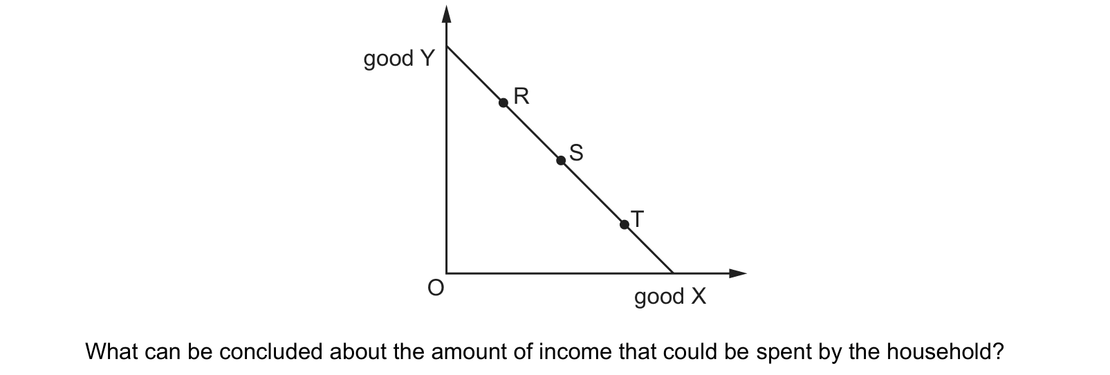
Answer: D.
Question 2
The diagram shows an individual’s indifference curve, I1, for apples and pears. 0 0 2 4 pears 19 12 apples X Y I1 What can be concluded from the movement from point X to point Y on this curve?
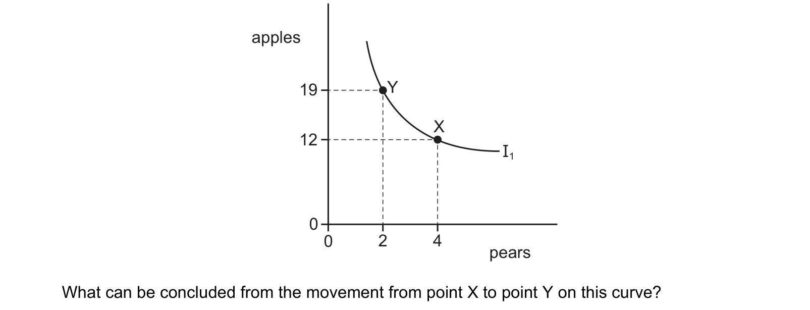
Answer: B.
The other options misread the diagram. Utility rises by moving to a HIGHER curve, not by sliding along one (D). Preference between the two goods (C) shows in the slope at a point rather than in the move itself. Affordability (A) depends on the budget line, which is not drawn here at all.
Question 3
To analyse a consumer’s preferences, an indifference curve represents possible combinations of goods X and Y.
The diagram shows a consumer’s indifference curve for good X and good Y. What can be concluded from the diagram?
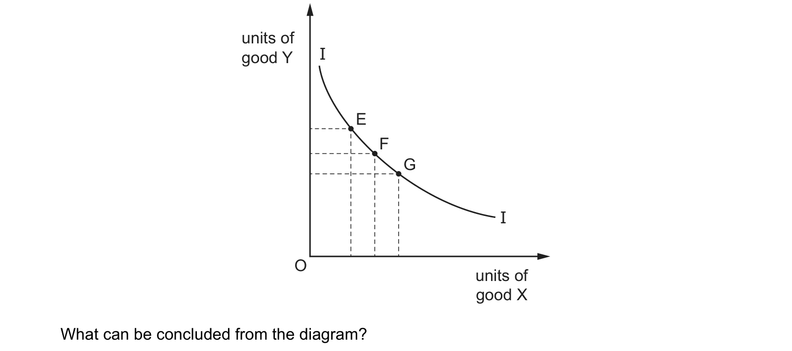
Answer: D.
25. Common exam mistakes
- Drawing two indifference curves that cross. Crossing curves break transitivity, so the map is invalid.
- Treating the numbers on indifference curves as measured utility. The ranking is ordinal, so only the order matters.
- Putting the optimum where an indifference curve cuts the budget line. The consumer can always reach a higher curve, so the optimum is the tangency.
- Reading the budget line slope as a statement about preferences. It is the ratio of the two prices.
- Reading the slope of an indifference curve as prices. It is the marginal rate of substitution, which reflects preferences.
- Pivoting the budget line when income changes. A change in income shifts it parallel; only a price change pivots it.
- Changing both intercepts when only one price changes.
- Calling the whole price effect the substitution effect, when it is the substitution effect plus the income effect.
- Drawing the compensated budget line parallel to the original rather than to the new one, or resting it on the new indifference curve rather than the original.
- Labelling every inferior good as Giffen. A Giffen good needs an income effect that outweighs the substitution effect.
- Confusing nominal income with real purchasing power when a price changes.
What the syllabus asks for on this topicCurrent Cambridge requirements
Current Cambridge requirements
This topic must cover:
- the meaning of an indifference curve and a budget line;
- causes of a change in the position of the budget line;
- income, substitution and price effects for normal, inferior and Giffen goods;
- limitations of the indifference-curve model.
Related CIE 9708 topics
Not the topic you were looking for? Describe what you are stuck on in your own words and we will take you to the notes that answer it.