Contents: 7 sections
Cambridge International AS & A Level Economics 9708 (A Level) Current syllabus: 2026–2028, Version 2 Official syllabus points: 7.1.1–7.1.5
Exam Essentials
1. Utility, total utility and marginal utility
Utility is the satisfaction or benefit a consumer obtains from consuming a good or service.
Utility is not the same as usefulness in an objective or moral sense. A product may provide utility to a consumer even when another person considers the choice unwise. Utility is therefore subjective.
Total utility (TU) is the total satisfaction gained from consuming a given quantity of a good or service during a stated period.
Marginal utility (MU) is the change in total utility produced by consuming one additional unit.
For a discrete change in quantity:
MU = change in TU / change in quantity
When quantity rises one unit at a time:
MU of the nth unit = TU at n units − TU at n − 1 units
Worked utility table
| Quantity consumed | Total utility | Marginal utility |
|---|---|---|
| 0 | 0 | : |
| 1 | 28 | 28 |
| 2 | 50 | 22 |
| 3 | 66 | 16 |
| 4 | 76 | 10 |
| 5 | 80 | 4 |
| 6 | 78 | −2 |
The sixth unit has negative marginal utility because total utility falls from 80 to 78.
Core relationships
- If MU is positive, TU rises.
- If MU is zero, TU is at a maximum, provided the next unit has negative MU.
- If MU is negative, TU falls.
- MU measures the slope or rate of change of TU.
A common error is to say that diminishing MU means TU must be falling. TU can still rise while MU is positive but falling. TU falls only when MU becomes negative.
Cardinal and ordinal utility
The simple marginal-utility model often treats utility as if it can be measured in numerical units, sometimes called “utils”. This is a cardinal interpretation.
In reality, consumers may be better able to rank choices than attach precise numerical utility scores to them. Ranking bundles from more preferred to less preferred is an ordinal interpretation. The difficulty of measuring cardinal utility is one of the theory’s limitations and motivates the indifference-curve approach in Topic 7.2.
2. Diminishing marginal utility
The law of diminishing marginal utility states that, other things equal, as a consumer consumes successive units of a good within a given period, the additional utility gained from each further unit tends to fall.

Example:
- the first bottle of water after exercise may provide very high MU;
- the second may still provide substantial MU;
- the fourth or fifth may provide much less;
- a further bottle may eventually produce discomfort and negative MU.
The law concerns marginal, not total, utility. Total utility normally continues to rise for as long as MU is positive, although it rises at a decreasing rate when MU is diminishing.
Why MU may diminish
Successive units are often used to satisfy less urgent wants. The first unit is allocated to the highest-value use, the next to a lower-value use, and so on. In addition, temporary satiation can reduce the satisfaction from repeated consumption in a short period.
Conditions and qualifications
Diminishing MU is not a mechanical rule that every consumer follows for every unit in every setting. The time period, indivisibility of goods, habit formation, collection effects, complementarities and changing circumstances can alter the pattern.
A learner should therefore state the ceteris paribus condition rather than treating the law as a universal physical law.
The equi-marginal principle
3. Utility maximisation across goods
Consumers have limited income and face prices. A rational consumer seeking to maximise total utility should compare the marginal utility gained per unit of currency spent on each good.
For goods X and Y, consumer equilibrium is represented by:
MUx / Px = MUy / Py
For several goods:
MUx / Px = MUy / Py = MUz / Pz = ...
subject to the consumer spending the available budget, where additional desirable units are divisible and available.
An equivalent two-good form is:
MUx / MUy = Px / Py
The marginal-utility-per-price form is usually more intuitive because it directly asks which purchase gives the larger extra satisfaction per pound, dollar or other currency unit.
The reallocation rule
- If MUx/Px > MUy/Py, shift spending towards X and away from Y.
- If MUx/Px < MUy/Py, shift spending towards Y and away from X.
- Reallocation continues until the ratios are equal, or as close as possible given indivisible units and the budget.
Worked example
A consumer currently buys the last unit of X with MU = 24 and price = £6, and the last unit of Y with MU = 15 and price = £5.
MUx/Px = 24/6 = 4 utils per £
MUy/Py = 15/5 = 3 utils per £
The last pound spent on X produces more utility. The consumer can raise total utility by shifting some spending from Y to X.
As more X is consumed, diminishing MU tends to lower MUx. As less Y is consumed, the MU of the last unit retained may rise. This process moves the consumer towards equality.
Budget exhaustion
Equality of MU/P is not sufficient if the consumer has unspent income that could purchase an additional unit with positive net benefit. In the standard model, the budget must also be fully allocated, assuming goods are desirable, divisible and there is no reason to hold money for future use.
Indivisible goods
With discrete units, exact equality may be impossible. The consumer chooses the affordable combination that gives the highest total utility. In an examination calculation, compare complete affordable bundles rather than forcing an impossible exact equality.
4. Calculating the utility-maximising allocation
Suppose a consumer has £12. Good A costs £4 per unit and Good B costs £2 per unit.
| Unit | MU from A | MU/P for A | MU from B | MU/P for B |
|---|---|---|---|---|
| 1 | 40 | 10 | 18 | 9 |
| 2 | 28 | 7 | 14 | 7 |
| 3 | 16 | 4 | 10 | 5 |
| 4 | 8 | 2 | 6 | 3 |
Rank purchasable units by MU per pound while respecting that the first unit must be bought before the second unit of the same good.
A utility-maximising allocation is:
- first unit of A: cost £4, MU 40;
- first unit of B: cost £2, MU 18;
- second unit of A: cost £4, MU 28;
- second unit of B: cost £2, MU 14.
Total cost = £12. Total utility = 100.
The last units purchased have equal MU/P of 7. The budget is exhausted.
Price changes
If the price of A falls while its marginal-utility schedule is unchanged, MUa/Pa rises at the existing quantity. The consumer has an incentive to buy more A. As additional units of A are consumed, MUa falls until equilibrium is restored.
This adjustment is central to deriving an individual demand curve.
Deriving an individual demand curve
5. From diminishing MU to willingness to pay
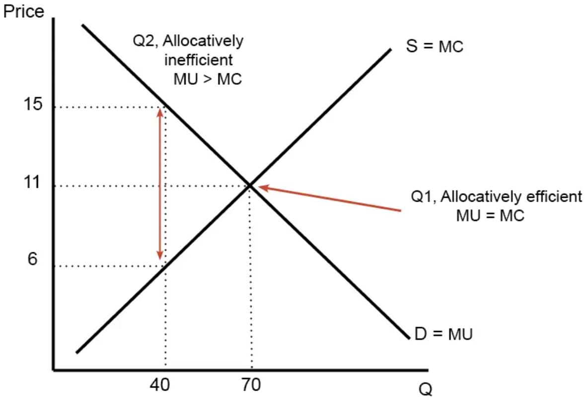
The marginal utility of each successive unit indicates the additional satisfaction obtained from that unit. If utility can be compared with the utility sacrificed by spending money, each unit has a maximum price the consumer is willing to pay.
Under the simple cardinal model, assume the marginal utility of money is constant. Let λ represent the marginal utility obtained from one unit of currency.
The consumer buys an additional unit when:
MU of the unit ≥ λ × price
At the margin, equilibrium is:
MU = λP
or:
MU/P = λ
Because MU normally diminishes as quantity rises, a lower price makes more units worth buying. This generates the inverse relationship between price and quantity demanded for the individual consumer.
Numerical derivation
Suppose the marginal utility of money is 2 utils per £ and successive units of a product provide MU of 20, 16, 12, 8 and 4 utils.
| Price | Utility cost per unit, λP | Quantity demanded |
|---|---|---|
| £10 | 20 | 1 |
| £8 | 16 | 2 |
| £6 | 12 | 3 |
| £4 | 8 | 4 |
| £2 | 4 | 5 |
Plotting price against quantity demanded gives an individual downward-sloping demand curve.
The causal chain
- price falls
- MU/P for the good rises at the original quantity
- the good gives more marginal utility per pound than alternatives
- spending shifts towards the good
- quantity demanded rises
- diminishing MU restores equilibrium
This is a derivation of the individual demand curve. Market demand is obtained later by horizontally summing the quantities demanded by all individuals at each price.
Important assumptions in the derivation
The simple derivation assumes:
- the marginal utility of money is constant;
- the utility from the good can be measured and compared with the utility of money;
- other prices, income, tastes and expectations are unchanged;
- units are sufficiently divisible;
- the consumer behaves consistently and seeks to maximise utility.
If these assumptions fail, the demand relationship may be less stable or harder to derive.
Rational behaviour and limitations
6. Assumptions of rational consumer behaviour
In the standard model, a rational consumer is assumed to:
- have preferences and be able to rank alternatives;
- behave consistently when faced with the same information and constraints;
- seek to maximise utility subject to income and prices;
- understand relevant prices, product characteristics and available alternatives;
- compare marginal benefits with marginal costs;
- adjust purchases when MU/P ratios differ;
- have stable preferences during the decision;
- face no serious calculation or information constraints.
“Rational” does not mean morally correct or selfish. It means internally consistent choice in pursuit of an objective under constraints.
7. Limitations of marginal utility theory
Utility is difficult to measure
Satisfaction cannot normally be observed directly or measured precisely in common units. Numerical utility schedules are useful analytical devices, but they should not be mistaken for directly recorded physical data.
Interpersonal comparisons are problematic
Even if one consumer assigns a number to satisfaction; it is difficult to compare that number meaningfully with another person’s utility.
Marginal utility of money may not be constant
Spending changes the amount of income remaining. The utility obtained from an extra pound may rise as the consumer becomes poorer. Large purchases make the constant-λ assumption especially questionable.
Preferences may be unstable or context-dependent
Advertising, framing, social norms, mood, defaults, habits and recent experiences can affect choices. Consumers may not have fixed preferences before the choice is presented.
Information is incomplete
Consumers may not know all prices, qualities, risks or future consequences. Search is costly, and firms may possess more information than buyers.
Calculation is demanding
Real consumers rarely calculate full marginal-utility schedules and MU/P ratios for every purchase. They use routines, rules of thumb and approximate comparisons.
Goods may not be independent
The utility of one good may depend on consumption of complements or substitutes. Coffee and milk, printers and ink, or streaming services and internet access cannot always be analysed as isolated utility schedules.
Indivisibility and fixed commitments
Housing, cars and annual subscriptions cannot be adjusted unit by unit. Exact equi-marginal equality may be impossible.
Behaviour may depart from consistency
Present bias, loss aversion, anchoring, status-quo bias and self-control problems can produce choices that differ from the simple rational-maximisation model.
Demand has other influences
Income effects, substitution effects, expectations, network effects, uncertainty and strategic behaviour can influence demand. Topic 7.2 develops an alternative consumer-choice model using budget lines and indifference curves.
8. Balanced evaluation
Marginal utility theory remains useful because it:
- focuses attention on decisions at the margin;
- explains why willingness to pay may fall for successive units;
- provides a clear rule for allocating limited income;
- offers one logical derivation of a downward-sloping individual demand curve;
- provides a benchmark against which real behaviour can be compared.
Its value is strongest as a simplified model rather than a literal description of every purchase. A good judgement recognises that models can be useful even when their assumptions are unrealistic, provided the assumptions are understood and the model gives testable or illuminating predictions.
Exam Mastery
9. Calculation method
For TU and MU tables:
- identify the change in quantity;
- calculate change in total utility;
- divide change in TU by change in quantity;
- keep the sign;
- explain what the sign implies for total utility.
For equi-marginal questions:
- calculate MU/P for each relevant marginal unit;
- identify the larger ratio;
- reallocate spending towards the larger ratio;
- account for diminishing MU;
- verify the budget is exhausted;
- with indivisible units, compare total utility of complete affordable bundles.
For demand derivation:
- state diminishing marginal utility;
- explain willingness to pay for successive units;
- hold marginal utility of money and other determinants constant;
- show that a lower price makes additional units worthwhile;
- conclude that quantity demanded rises as price falls.
10. Common exam traps
- Confusing TU with MU.
- Saying falling MU means falling TU.
- Omitting the change in quantity from the MU formula.
- Comparing MU alone instead of MU/P when prices differ.
- Giving the ratio MUx/MUy = Px/Py without explaining reallocation.
- Forgetting the budget constraint.
- Treating exact equality as compulsory when goods are indivisible.
- Deriving market demand when the syllabus asks for an individual demand curve.
- Reversing the conventional axes: price belongs on the vertical axis and quantity on the horizontal axis.
- Claiming that consumers literally calculate “utils”.
- Calling every unexpected choice irrational without identifying the objective, information and constraint.
Check you have it
Question 1
To maximise the satisfaction he derives from a given level of expenditure on two goods, X and Y, a consumer should allocate his expenditure between the two goods so that
Answer: D.
Question 2
To maximise the satisfaction she derives from a given level of expenditure on two goods, X and Y, how should a consumer allocate her expenditure between the two goods?
Answer: D.
Question 3
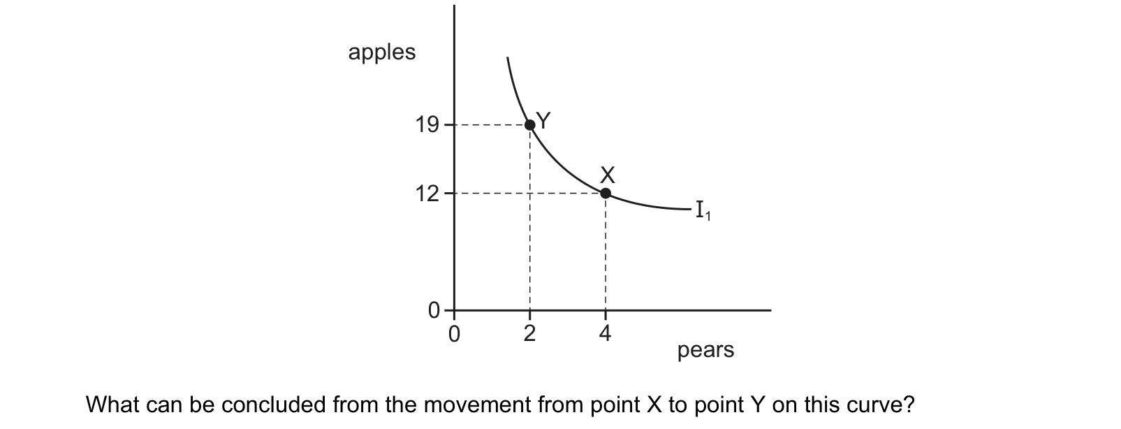
The diagram shows an individual’s indifference curve, I1, for apples and pears. 0 0 2 4 pears 19 12 apples X Y I1 What can be concluded from the movement from point X to point Y on this curve?
Answer: B.
The other options misread the diagram. Utility rises by moving to a HIGHER curve, not by sliding along one (D). Preference between the two goods (C) shows in the slope at a point rather than in the move itself. Affordability (A) depends on the budget line, which is not drawn here at all.
11. Syllabus boundary
Topic 7.1 requires marginal utility theory and its limitations. Detailed indifference-curve analysis, budget-line shifts, income/substitution effects and Giffen goods belong to Topic 7.2.
Behavioural concepts can enrich evaluation of rationality, but detailed named-theory coverage is not a separate current syllabus requirement. Use behavioural examples to assess assumptions rather than allowing them to replace the required utility analysis.
Final checklist
A learner is secure when they can:
- define utility, TU and MU precisely;
- calculate MU from a TU schedule and reconstruct TU from MU;
- explain TU when MU is positive, zero or negative;
- apply diminishing marginal utility with a ceteris paribus qualification;
- use MU/P to identify a better allocation;
- find the utility-maximising affordable bundle;
- derive an individual demand curve from diminishing MU and price changes;
- state assumptions of rational behaviour;
- evaluate marginal utility theory without dismissing its analytical usefulness.
What the syllabus asks for on this topicCurrent Cambridge requirements
Current Cambridge requirements
This topic must cover:
- the definition and calculation of total utility and marginal utility;
- diminishing marginal utility;
- the equi-marginal principle;
- derivation of an individual demand curve;
- limitations of marginal utility theory and its assumptions of rational behaviour.

Related CIE 9708 topics
Not the topic you were looking for? Describe what you are stuck on in your own words and we will take you to the notes that answer it.