The Circular Flow, Injections and Withdrawals
National Income Equilibrium and the Conditions for Change
Contents: 17 sections
1. Why this topic matters
At AS Level the circular flow was a description: households supply factors, firms pay incomes, households spend. At A2 it becomes an equilibrium model that explains why national income settles where it does and what makes it move.
Everything in the rest of chapter 9 rests on this. The multiplier in 9.2 is derived from the withdrawals in this topic. The Keynesian aggregate supply curve in 9.3 depends on whether the economy is below or at full capacity, which is a statement about this equilibrium. The interest rate in 9.5 matters because it changes two of the flows described here.
The central result to master is that national income is in equilibrium where planned injections equal planned withdrawals, and that this equilibrium need not be at full employment. That last clause is the whole Keynesian contribution and it is examined constantly.
2. The flows
2.1 The two-sector model
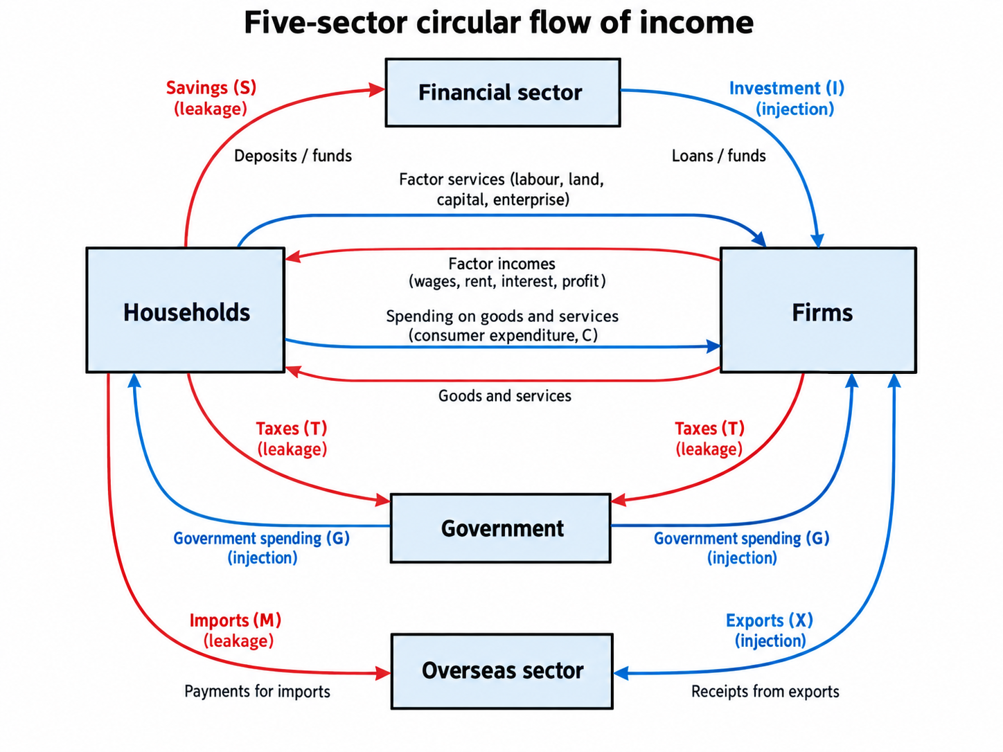
In the simplest model there are only households and firms.
- Households supply factors of production and receive income (Y).
- Households spend that income on goods and services, which is consumption (C).
- Firms receive that spending as revenue and pay it out again as factor incomes.
If households spend all their income, the flow is self-sustaining and income is constant.
2.2 Withdrawals
A withdrawal (or leakage) is income received by households that is not passed back to domestic firms as spending on domestic output. There are three:
- Saving (S): income not spent.
- Taxation (T): income taken by the government.
- Imports (M): spending that flows to foreign producers rather than domestic ones.
Total withdrawals: W equals S plus T plus M.
2.3 Injections
An injection is spending on domestic output that does not come from domestic household income. There are three:
- Investment (I): firms' spending on capital goods.
- Government spending (G): on goods and services.
- Exports (X): foreign spending on domestic output.
Total injections: J equals I plus G plus X.
2.4 The pairing is not a matching
Students often assume saving funds investment, tax funds government spending and imports are paid for by exports, so each pair cancels. They do not, because different people make the decisions for different reasons.
Households decide to save based on income, interest rates and confidence. Firms decide to invest based on expected returns and the cost of borrowing. There is no mechanism guaranteeing the two plans coincide. The same applies to the other two pairs.
That independence is precisely why national income can settle below full employment, and it is the analytical heart of this topic.
3. Equilibrium national income
3.1 The condition
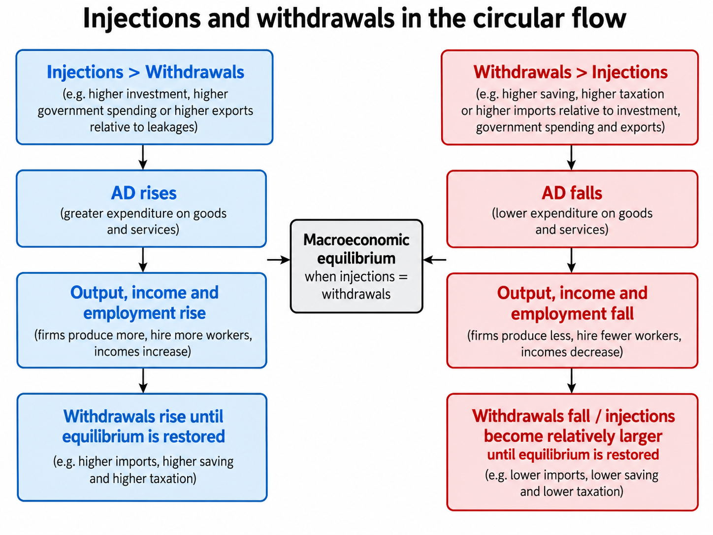
National income is in equilibrium where planned injections equal planned withdrawals:
I plus G plus X equals S plus T plus M
Equivalently, in the expenditure form, equilibrium occurs where planned aggregate expenditure equals national output:
Y equals C plus I plus G plus (X minus M)
3.2 Why the economy moves towards it
Suppose planned injections exceed planned withdrawals.
- More is being spent on domestic output than is being withdrawn from the flow.
- Firms find stocks falling faster than expected, so they raise output and employment.
- Higher output means higher incomes, which raises consumption, and also raises saving, tax and imports.
- Withdrawals rise until they equal injections, and income stops changing.
Now suppose planned withdrawals exceed planned injections.
- Spending on domestic output is less than the income leaking out.
- Firms accumulate unsold stocks, so they cut output and employment.
- Income falls, which reduces saving, tax and imports.
- Withdrawals fall until they equal injections.
The adjustment mechanism is changes in output and income, not changes in price. That is the Keynesian assumption, and it is why it applies most convincingly when there is spare capacity.
3.3 Worked example
An economy has planned investment of $40 billion, government spending of $70 billion and exports of $50 billion, so injections total $160 billion.
At the current income level, planned saving is $45 billion, tax revenue $80 billion and imports $60 billion, so withdrawals total $185 billion.
Withdrawals exceed injections by $25 billion. Firms will find stocks rising, so output and income will fall until withdrawals have fallen by $25 billion. The economy contracts.
Note carefully what this does not say. It does not say the economy moves to full employment. It says it moves to the income level at which withdrawals equal $160 billion, wherever that happens to be.
4. Equilibrium below full employment
4.1 The central Keynesian claim
The equilibrium described above is a level of income at which the economy is stable, meaning there is no tendency to change. It is not necessarily the level at which everyone who wants work has it.
If the equilibrium income is below the full employment level, the difference is called a deflationary gap (or output gap): the shortfall of aggregate demand below what is needed to buy the full employment level of output. Unemployment persists, and there is no automatic mechanism returning the economy to full employment quickly.
If planned expenditure exceeds what the economy can produce at full employment, the excess is an inflationary gap, and the result is a rise in the price level rather than in real output.
4.2 Why this matters for policy
If the economy self-corrected reliably, discretionary demand management would be unnecessary. The claim that it may not is the justification for fiscal policy as a stabilisation tool, which is chapter 10's subject.
The classical response, developed in 9.3, is that wages and prices adjust so that the economy does return to full employment, and that the only question is how quickly.
5. The consumption function
5.1 Consumption and income
Keynes proposed that consumption depends primarily on current disposable income:
C equals a plus bYd
where a is autonomous consumption, the amount consumed at zero income, funded by dissaving or borrowing, and b is the marginal propensity to consume.
5.2 Propensities
- Marginal propensity to consume (MPC) is the fraction of each additional unit of income that is spent: change in C divided by change in Y.
- Average propensity to consume (APC) is total consumption divided by total income.
- Marginal propensity to save (MPS) is the fraction of extra income saved.
In a closed economy with no government, MPC plus MPS equals 1, since each extra dollar is either spent or saved.
In an open economy with government, each extra dollar of income is either consumed domestically or withdrawn, so:
MPC plus MPS plus MPT plus MPM equals 1
where MPT is the marginal propensity to tax and MPM the marginal propensity to import.
The marginal propensity to withdraw (MPW) equals MPS plus MPT plus MPM, and MPC plus MPW equals 1.
5.3 Worked calculation
Income rises by $500. Of that, $60 is saved, $90 goes in tax and $50 is spent on imports.
- MPS equals 60 divided by 500, which is 0.12.
- MPT equals 90 divided by 500, which is 0.18.
- MPM equals 50 divided by 500, which is 0.10.
- MPW equals 0.12 plus 0.18 plus 0.10, which is 0.40.
- MPC equals 1 minus 0.40, which is 0.60.
Check: consumption of domestic output rises by 0.60 multiplied by $500, which is $300, and $300 plus $60 plus $90 plus $50 equals $500.
These figures feed directly into the multiplier in 9.2, so being fluent with them is essential.
5.4 Other influences on consumption
Beyond current income:
- Wealth, since rising asset values encourage spending;
- Interest rates, which change the cost of borrowing and the reward for saving;
- Expectations and confidence about future income and job security;
- Availability of credit; and
- The distribution of income, because poorer households have a higher MPC, so redistribution towards them raises aggregate consumption. This links directly to 8.2.
6. Investment
Investment is the most volatile injection, and its determinants are examinable.
- The rate of interest, since it is the cost of borrowing and the opportunity cost of using retained profit.
- Expected returns and business confidence, which Keynes called animal spirits. Expectations are volatile and self-reinforcing, which is why investment fluctuates far more than consumption.
- The rate of change of national income, which is the accelerator, covered in 9.2.
- Technological change, which creates new profitable opportunities.
- Corporate taxation and investment allowances.
- The existing capital stock and spare capacity, since firms with idle capital have little reason to add more.
7. The classical position
11.1 The aggregate supply curve
The classical long run aggregate supply (LRAS) curve is vertical at the full employment level of output, sometimes labelled the potential output or Yf.
The reasoning is that real output depends on real factors: the quantity and quality of labour, capital, land and enterprise, and the technology available. It does not depend on the price level. Doubling all prices and all wages leaves the real incentives to produce unchanged, so it leaves output unchanged.
11.2 Why the economy self-corrects
Suppose aggregate demand falls, so output falls below full employment and unemployment rises.
- The surplus of labour bids wages down.
- Falling wages reduce firms' costs, so they are willing to supply more at every price level.
- Prices fall, real balances rise, and output returns to Yf.
The adjustment happens through prices and wages, not through a permanent change in output. Unemployment above the natural rate is therefore temporary and self-correcting.
11.3 The policy conclusion
An increase in aggregate demand in the long run raises the price level only, leaving real output unchanged. Demand management is therefore inflationary and futile.
To raise output, the government must shift LRAS rightward, which requires supply-side policy: improving education and training, incentives to work and invest, competition, infrastructure and labour market flexibility.
11.4 The assumptions it rests on
- Wages and prices are flexible in both directions.
- Markets clear.
- Agents are rational and reasonably well informed.
- There is no persistent coordination failure.
Each is a point of attack in an evaluation.
8. The Keynesian position
11.1 The aggregate supply curve
The Keynesian AS curve has three sections, and being able to explain each is essential.
- A perfectly elastic (horizontal) section at low levels of output. There is substantial spare capacity and heavy unemployment, so firms can hire more labour and raise output without bidding up wages or costs. Extra demand raises real output with no effect on the price level.
- An upward sloping section as output approaches capacity. Bottlenecks appear: skilled labour becomes scarce in some sectors, less efficient capital is brought into use, and firms pay overtime. Costs rise, so extra demand raises both output and the price level.
- A perfectly inelastic (vertical) section at full capacity. No further real output is possible, so extra demand raises the price level only.
Note that the Keynesian curve contains the classical result as its final section. The disagreement is about where the economy typically sits, not about whether a capacity limit exists.
11.2 Why the economy may not self-correct
Keynes argued that wages are sticky downwards. They do not fall readily when unemployment rises, because:
- workers resist nominal wage cuts, and contracts and collective agreements fix wages for periods;
- employers avoid cuts because they damage morale and productivity and cause the best workers to leave; and
- minimum wages and employment protection set floors.
If wages do not fall, the classical adjustment mechanism does not operate, and the economy can remain at an equilibrium below full employment indefinitely. This is the deflationary gap from 9.1.
11.3 The paradox of thrift
Even where wages do fall, Keynes identified a mechanism that can make matters worse. If households respond to uncertainty by saving more, consumption falls, so aggregate demand falls, so income falls. Because saving depends on income, total saving may end up no higher, or even lower, than before.
What is rational for one household is damaging when all households do it together. This is a coordination failure, and it is an argument that the government must act because no individual agent can.
11.4 The policy conclusion
Where the economy sits on the horizontal or gently sloping section, an increase in aggregate demand raises real output and employment with little or no inflation. Fiscal policy is therefore effective, and the multiplier from 9.2 magnifies the effect.
9. Comparing the two directly
| Classical | Keynesian | |
|---|---|---|
| Shape of AS | Vertical at Yf | Horizontal, then rising, then vertical |
| Wage flexibility | Flexible both ways | Sticky downwards |
| Does the economy self-correct? | Yes, and reasonably quickly | Not reliably, and possibly not at all |
| Effect of a rise in AD | Price level only | Output, or output and prices, or prices only, depending on the section |
| Unemployment above the natural rate | Temporary | Can persist |
| Preferred policy | Supply-side | Demand management, then supply-side |
| Role for government | Minimal, set the framework | Active stabilisation |
11.1 The synthesis
The distinction is best presented as one about time and circumstance rather than about right and wrong.
Most economists accept that the Keynesian analysis describes the short run, in which prices and wages are sticky, and that the classical analysis describes the long run, in which they have had time to adjust. Keynes's own reply to the argument that markets clear eventually was that the long run is a misleading guide to current affairs, because in the long run we are all dead.
An answer that reaches this synthesis, and then says which analysis fits the case in the question, is doing exactly what the evaluation marks reward.
10. Applying it to a specific case
11.1 A deflationary gap
Aggregate demand is low, the economy sits on the horizontal section, unemployment is 11 per cent and inflation is close to zero.
- Keynesian analysis: a fiscal expansion raises real output substantially with little inflation. The multiplier operates fully because there is spare capacity. Intervention is justified.
- Classical analysis: wages will fall, restoring full employment without intervention. The fiscal expansion will raise borrowing, crowd out private investment and eventually raise prices.
- Judgement: the Keynesian case is stronger where wages have visibly failed to fall over several years and the output gap is large and persistent. The classical warning about crowding out remains relevant if the economy recovers faster than the policy takes effect, which is the time lag problem from 8.4.
11.2 Near full capacity
Unemployment is 4 per cent, close to the natural rate, and inflation is 6 per cent.
- Both analyses agree here. The economy is on or near the vertical section, so extra demand raises prices with little real gain.
- The appropriate policy is supply-side, aimed at shifting the capacity constraint rather than pushing against it.
Recognising that the two schools agree in this case is a strong move, because it shows the disagreement is conditional rather than absolute.
11. The natural rate and the vertical long run
Classical and monetarist analysis holds that there is a natural rate of unemployment, determined by the structure of the labour market rather than by demand. It consists of frictional and structural unemployment and is the rate consistent with stable inflation.
Attempts to push unemployment below the natural rate by raising demand succeed only while people are fooled by rising prices into thinking real wages have risen. Once expectations adjust, unemployment returns to the natural rate at a higher rate of inflation. This is the expectations-augmented Phillips curve, developed in 9.6.
The policy implication is that only supply-side measures which change the structure of the labour market can reduce unemployment permanently.
12. The multiplier
14.1 The idea
An injection is spent, and the recipient's income rises. That recipient spends part of the increase, which becomes someone else's income, who spends part again. Each round is smaller than the last because part of every increase leaks out as saving, tax and imports.
The total rise in income is therefore a multiple of the original injection.
14.2 Definition
The multiplier (k) is the ratio of the final change in national income to the initial change in an injection:
k equals change in Y divided by change in J
14.3 The formulae
In a closed economy with no government:
k equals 1 divided by MPS, or equivalently 1 divided by (1 minus MPC)
In an open economy with government:
k equals 1 divided by MPW, where MPW equals MPS plus MPT plus MPM
The general and always correct form is:
k equals 1 divided by the marginal propensity to withdraw
Use that one. The simpler version is a special case in which two of the withdrawals are zero, and using it on an open economy question is the single most common error in this topic.
14.4 Worked calculation
An economy has MPS of 0.15, MPT of 0.20 and MPM of 0.05. The government raises spending by $8 billion.
- MPW equals 0.15 plus 0.20 plus 0.05, which is 0.40.
- k equals 1 divided by 0.40, which is 2.5.
- Change in Y equals 2.5 multiplied by $8 billion, which is $20 billion.
Note that MPC is 0.60 here. A student who wrongly used 1 divided by (1 minus MPC) would get 1 divided by 0.40, which is the same answer only because MPC and MPW happen to sum to 1 by construction. The formulae agree; the danger is using 1 divided by MPS alone, which would give 6.67 and overstate the effect by more than two and a half times.
14.5 The rounds, traced
Take an injection of $1,000 with MPW of 0.4, so 60 per cent of each increase is passed on.
| Round | Extra spending | Cumulative income |
|---|---|---|
| 1 | $1,000 | $1,000 |
| 2 | $600 | $1,600 |
| 3 | $360 | $1,960 |
| 4 | $216 | $2,176 |
| 5 | $130 | $2,306 |
The series converges on $1,000 divided by 0.4, which is $2,500. Each round is 60 per cent of the last, so the increments shrink geometrically and the total is finite.
Being able to show two or three rounds is worth more than quoting the formula, because it demonstrates the mechanism.
14.6 What makes the multiplier large or small
The multiplier is larger when the marginal propensity to withdraw is small, meaning more of each round is passed on:
- low marginal propensity to save;
- low marginal tax rate; and
- low marginal propensity to import.
It follows that:
- Small open economies have small multipliers, because a high MPM means much of each round leaks abroad. This is a reliable evaluation point when a question concerns a country heavily dependent on trade.
- Progressive tax systems reduce the multiplier, because MPT rises with income. This is why they act as automatic stabilisers, damping both booms and slumps.
- Redistribution towards low income households raises the multiplier, because their MPC is higher.
14.7 The negative multiplier
The process works identically in reverse. A fall in injections produces a magnified fall in income. A withdrawal of $5 billion of government spending with MPW of 0.25 reduces income by $20 billion.
This symmetry is why sharp fiscal contraction during a downturn can deepen it, and it is the core of the argument about austerity.
14.8 Limitations
The simple multiplier assumes:
- spare capacity, so that extra demand raises output rather than prices. At or near full employment the multiplier effect appears as inflation instead, and the real multiplier approaches zero;
- no crowding out, whereas government borrowing may raise interest rates and displace private investment;
- constant propensities, whereas they vary with income and confidence;
- no change in expectations, whereas households anticipating future tax rises may save the increase; and
- no time lags, whereas the rounds take quarters or years, so the full effect may arrive after the conditions have changed.
Each of these is an evaluation point, and each turns on a condition that can be checked against the case in the question.
13. The accelerator
14.1 The idea
The accelerator states that investment depends on the rate of change of national income rather than its level.
The reasoning is about the capital stock. Firms hold capital in some proportion to the output they expect to produce. If output is constant, they need only replace worn out capital. To raise output; they must add to the capital stock, which requires investment above replacement.
14.2 The capital-output ratio
If the desired capital-output ratio is v, then desired capital equals v multiplied by expected output, and net investment equals v multiplied by the change in output.
14.3 Worked calculation
A firm needs $4 of capital for every $1 of annual output, so v equals 4. Its capital stock lasts ten years, so replacement investment is 10 per cent of the stock each year.
| Year | Output | Required capital | Net investment | Replacement | Gross investment |
|---|---|---|---|---|---|
| 1 | $100 | $400 | 0 | $40 | $40 |
| 2 | $110 | $440 | $40 | $40 | $80 |
| 3 | $115 | $460 | $20 | $44 | $64 |
| 4 | $115 | $460 | 0 | $46 | $46 |
Read the third and fourth rows carefully, because they contain the examinable insight.
Between years 2 and 3, output is still rising, from $110 to $115, yet gross investment falls from $80 to $64. Investment fell because output rose by less than before. Between years 3 and 4 output stops growing and net investment falls to zero.
So a mere slowdown in the growth of demand causes an absolute fall in investment. That is the accelerator, and it explains why capital goods industries suffer far sharper cycles than consumer goods industries.
14.4 Limitations
- Firms with spare capacity can raise output without investing, so the accelerator is weak in a downturn.
- Investment decisions rest on expected future output, not merely on the last change, and firms may treat a change as temporary.
- Time lags in ordering and installing capital blur the relationship.
- The capital-output ratio is not fixed, since technology changes it.
- Firms may be unable to finance the investment even when they want it.
14. The multiplier and accelerator together
The interaction generates cycles.
An initial injection raises income through the multiplier. Rising income raises investment through the accelerator. That investment is itself an injection, so it raises income again through the multiplier, which raises investment again. The upswing is self-reinforcing.
The process cannot continue indefinitely. As the economy approaches capacity, output growth slows. Because the accelerator depends on the rate of change, slowing growth causes investment to fall absolutely, which reduces income through the multiplier, which reduces investment further. The downswing is equally self-reinforcing.
This interaction is the standard explanation of the business cycle in this syllabus, and being able to state why the turning points occur, rather than merely that they do, is what distinguishes a strong answer.
15. Integrated analysis and common traps
7.1 A complete chain
A fall in business confidence reduces planned investment by $10 billion. Injections now fall short of withdrawals, so firms accumulate stocks and cut output. Income falls, and as it does, saving, tax revenue and import spending all fall. Income continues to fall until withdrawals have contracted by the full $10 billion. The size of the total fall depends on the marginal propensity to withdraw: the smaller the MPW, the further income must fall before withdrawals contract enough, which is the multiplier from 9.2.
The economy is then in equilibrium again, at a lower income, with higher unemployment, and with no automatic force returning it to the previous level.
7.2 Common examination errors
- Assuming saving must equal investment because both appear in the model. Planned saving and planned investment are decided by different agents and need not be equal; it is the adjustment of income that brings them into line.
- Treating equilibrium as full employment.
- Classifying a transfer payment as a government injection. Transfers are not spending on goods and services; they redistribute income and affect the flow through consumption instead.
- Forgetting that imports are a withdrawal and exports an injection, and reversing them.
- Confusing average and marginal propensities.
- Saying the adjustment happens through prices when the Keynesian mechanism is through output.
16. Paper 3 and Paper 4 mastery
Paper 3 tests: identifying which items are injections and which withdrawals, computing propensities from a table, and determining the direction of income change when J and W differ.
Paper 4 uses this model as the foundation for demand management essays. The strong move is to state the equilibrium condition. Show why equilibrium can sit below full employment, and only then discuss policy, because that sequence establishes why intervention might be needed at all.
Be precise about the word planned. Actual saving and actual investment are equal after the event by accounting identity; it is the equality of planned magnitudes that defines equilibrium.
Check you have it
Question 1
In a closed economy with no government sector, when will an increase in investment spending generate the largest increase in equilibrium national income?
Answer: C.
Question 2
The government cuts taxes and increases its spending in order to create jobs during a recession. When will a resulting budget deficit be least likely to cause a permanent reduction in unemployment?
Answer: A.
Question 3
In a 4-sector economy, consisting of households, firms, government and foreign trade, the level of national income is in equilibrium where C + I + G + (X – M) = Y. What must Y include for an equilibrium to exist?
Answer: B.
17. Final checklist
A fully prepared learner can:
- list the three injections and three withdrawals and classify a given flow correctly;
- explain why the pairs are decided independently and what follows from that;
- state the equilibrium condition in both the injections equals withdrawals and expenditure forms;
- explain the adjustment mechanism through stocks, output and income in both directions;
- work out the direction of change from given values of J and W;
- explain why equilibrium may lie below full employment and define a deflationary gap;
- write the consumption function and define autonomous consumption;
- calculate MPC, MPS, MPT, MPM and MPW from a change in income;
- state that MPC plus MPW equals 1 and verify it numerically;
- list the determinants of consumption and of investment; and
- explain why transfer payments are not counted as an injection.
Related CIE 9708 topics
Not the topic you were looking for? Describe what you are stuck on in your own words and we will take you to the notes that answer it.