Externalities and Social Costs and Benefits
Private Costs and Benefits, Externalities and Social Costs and Benefits
Contents: 20 sections
1. Why this topic matters
Markets coordinate decisions through prices, but market prices do not always contain every cost or benefit created by an activity. A buyer and seller may consider their own gains and losses while effects on other people remain outside the transaction. Topic 7.4 provides the language and marginal analysis needed to identify that gap.
The central comparison is:
market output, determined by private costs and private benefits, versus socially efficient output, determined by social costs and social benefits.
This topic is not simply a list of pollution examples. It requires accurate definitions, calculations, four distinct externality diagrams, welfare-loss analysis, information failure and the disciplined use of costs and benefits in decision-making.
2. Private, external and social costs
2.1 Private cost
A private cost is a cost borne by the decision-maker directly involved in production or consumption.
For a producer, private costs can include wages, raw materials, rent, energy bills and the opportunity cost of owner-supplied resources. For a consumer, private costs can include the price paid, travel time or other direct sacrifices made to consume a product.
2.2 External cost
An external cost is an uncompensated cost imposed on a third party who is not directly involved in the relevant market transaction.
Examples include:
- respiratory harm experienced by nearby residents because of factory emissions;
- sleep disturbance caused by aircraft noise;
- congestion imposed on other road users by an additional car journey;
- second-hand smoke affecting non-smokers.
An effect is not external merely because it is unpleasant. It must fall on a third party and be insufficiently reflected in the decision-maker's private incentives or the market price.
2.3 Social cost
Social cost is the total cost to society:
SC = PC + EC
At the margin:
MSC = MPC + MEC
where:
- MPC is the private cost of one additional unit;
- MEC is the external cost of one additional unit;
- MSC is the total social cost of one additional unit.
Worked calculation
A delivery company's additional journey costs it $38 in fuel, labour and vehicle wear. The journey creates estimated congestion and pollution costs of $14 for other people.
- MPC = $38
- MEC = $14
- MSC = $38 + $14 = $52
A common error is to subtract external cost from private cost. The external cost is an additional cost borne elsewhere, so it is added.
2.4 The vertical distance between curves
On a marginal diagram, the vertical distance between MSC and MPC at a particular output equals MEC at that output:
MEC = MSC − MPC
The distance does not have to be constant. The syllabus does not require the assumption that external cost rises proportionately or disproportionately with output. The curve shape should follow the information given.
3. Private, external and social benefits
3.1 Private benefit
A private benefit is a benefit received by the individual or firm directly involved in an activity.
For a consumer; it may be the satisfaction, convenience or earnings benefit obtained from consuming a product. For a producer; it may include revenue or productivity gains received by the firm.
3.2 External benefit
An external benefit is an uncompensated benefit received by a third party who is not directly involved in the market transaction.
Examples include:
- lower infection risk for other people when an individual receives a vaccination;
- knowledge spillovers to other firms from research and worker training;
- improved neighbourhood appearance when a property owner restores a historic building;
- reduced congestion and emissions when a commuter cycles rather than drives.
3.3 Social benefit
Social benefit is the total benefit to society:
SB = PB + EB
At the margin:
MSB = MPB + MEB
where:
- MPB is the private benefit of one additional unit;
- MEB is the external benefit of one additional unit;
- MSB is the total social benefit of one additional unit.
Worked calculation
A training course gives the participant an estimated private benefit of $900 and creates a $350 productivity spillover for colleagues and future employers.
- PB = $900
- EB = $350
- SB = $1,250
At a particular output, the vertical distance between MSB and MPB is MEB:
MEB = MSB − MPB
4. Positive and negative externalities
An externality exists when production or consumption affects a third party and the effect is not fully reflected in market prices or compensation.
- A negative externality imposes an external cost.
- A positive externality creates an external benefit.
The words positive and negative refer to the spillover, not to whether the entire product is morally good or bad. A product may provide substantial private benefit while also creating a negative externality. Likewise, a profitable activity can create external benefits.
Externalities must also be separated from merit and demerit goods. Merit and demerit analysis often focuses on imperfect information and consumers undervaluing or overvaluing private benefits or costs. Externalities focus on third-party effects. The two problems can occur together, but they are not synonyms.
5. Market equilibrium and the social optimum
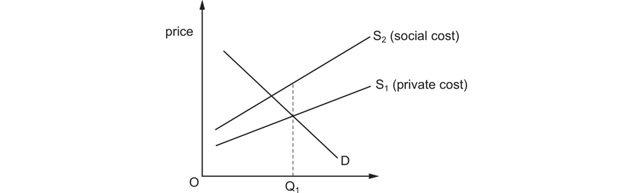
In a simplified competitive market:
- market demand represents MPB;
- market supply represents MPC;
- market equilibrium occurs where MPB = MPC.
The socially efficient output occurs where:
MSB = MSC
At this point, the social benefit from the last unit equals the social cost of producing or consuming it. Producing one more unit would add more social cost than benefit; producing one fewer would sacrifice a unit whose social benefit exceeds its social cost.
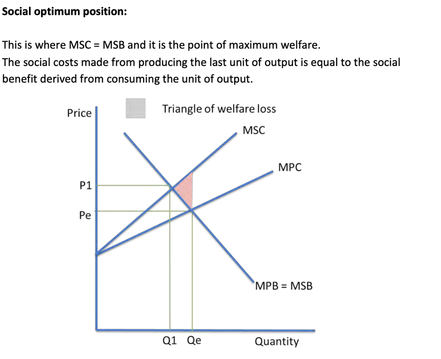
When private and social values coincide, MPB = MSB and MPC = MSC, the competitive market equilibrium can also be socially efficient. Externalities create a divergence between the private and social curves.
6. Negative externality of production
6.1 Economic structure
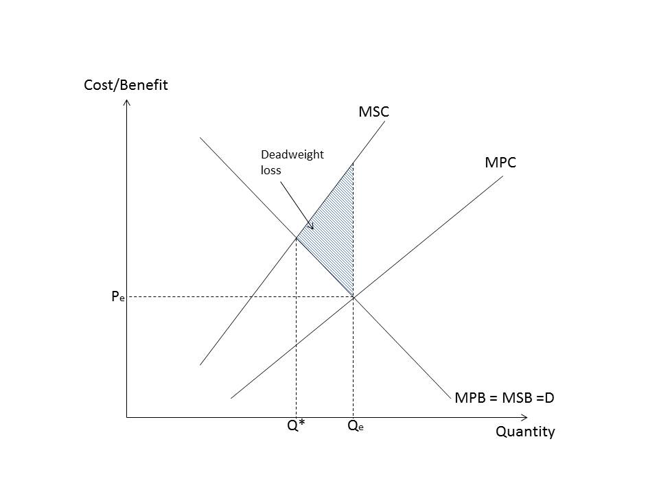
A negative production externality occurs when producing a good imposes an external cost on third parties.
Typical simplified assumptions:
- MSC > MPC because MEC is positive;
- MPB = MSB if consumption creates no externality.
The market equilibrium is where MPB = MPC. Because producers do not bear the whole social cost, market output is too high:
Qmarket > Qsocial
The social optimum is where MSB = MSC.
6.2 Causal chain
Factory output rises → the firm considers its own marginal production cost → pollution damage borne by residents is not fully priced → MPC understates MSC → the market produces beyond the point where MSB = MSC → resources are overallocated to the good.
6.3 Diagram discipline
A correct diagram should show:
- quantity on the horizontal axis and cost/benefit on the vertical axis;
- an upward-sloping MPC curve;
- an MSC curve above MPC;
- a downward-sloping MPB = MSB curve;
- market output at MPC = MPB;
- social output at MSC = MSB;
- Qmarket to the right of Qsocial;
- welfare loss between MSC and MSB over the excess units from Qsocial to Qmarket.
Do not label the full vertical distance between MSC and MPC as welfare loss. That distance is MEC. Welfare loss is the sum of the marginal social losses on the excess units.
7. Negative externality of consumption
7.1 Economic structure
A negative consumption externality occurs when consuming a good imposes costs on third parties.
Typical simplified assumptions:
- MPB > MSB because consumption creates an external cost or negative external benefit;
- MPC = MSC if production creates no externality.
Consumers base demand on private benefit and therefore demand more than is socially efficient:
Qmarket > Qsocial
7.2 Example
A driver may receive the private convenience of a car journey while imposing congestion, noise and emissions on others. If those third-party costs are not fully faced by the driver, MPB overstates MSB.
7.3 Diagram discipline
The demand-side divergence is crucial:
- MPB is above MSB;
- MPC = MSC is the supply curve;
- market output is MPB = MPC;
- social output is MSB = MSC;
- the welfare-loss region covers the overconsumed units between Qsocial and Qmarket.
Do not automatically describe every demerit good as a negative consumption externality. A consumer may overconsume because of imperfect information even if no third party is affected.
8. Positive externality of production
8.1 Economic structure
A positive production externality occurs when production creates benefits for third parties.
Examples include knowledge spillovers from research, worker training that raises wider industry productivity, or environmental improvements generated by a firm's production process.
A standard way to represent this is:
- MSC < MPC, because external production benefits reduce the net social cost of additional output;
- MPB = MSB, if consumption creates no externality.
The market output is too low:
Qmarket < Qsocial
8.2 Why MSC can lie below MPC
The firm bears MPC, but society receives an additional external benefit from production. That benefit can be treated as reducing the net social cost:
MSC = MPC − marginal external production benefit
This is consistent with the general social-benefit framework, but the diagram must state clearly what is being represented. Avoid switching curve conventions halfway through an answer.
8.3 Diagram discipline
- MPC lies above MSC;
- MPB = MSB slopes downward;
- market output is MPC = MPB;
- social output is MSC = MSB;
- Qsocial lies to the right of Qmarket;
- welfare loss covers the beneficial units forgone between Qmarket and Qsocial, where MSB exceeds MSC.
9. Positive externality of consumption
9.1 Economic structure
A positive consumption externality occurs when consumption provides benefits to third parties.
Typical simplified assumptions:
- MSB > MPB because MEB is positive;
- MSC = MPC if production creates no externality.
The market underconsumes the good:
Qmarket < Qsocial
Vaccination is a common example. The vaccinated person gains private health protection, while other people benefit from a reduced probability of transmission.
9.2 Diagram discipline
- MSB lies above MPB;
- MSC = MPC is upward sloping;
- market output occurs where MPB = MPC;
- social output occurs where MSB = MSC;
- welfare loss lies over the missing units from Qmarket to Qsocial, where MSB exceeds MSC.
10. Deadweight welfare loss
A deadweight welfare loss is the net social benefit lost because output differs from the socially efficient level.
It is not a transfer from one group to another. A transfer changes who receives welfare; deadweight loss represents welfare that no one receives.
10.1 Overproduction or overconsumption
For units beyond Qsocial:
MSC > MSB
Each excess unit creates a marginal social loss of:
MSC − MSB
The welfare-loss area is the sum of those losses from Qsocial to Qmarket.
10.2 Underproduction or underconsumption
For units between Qmarket and Qsocial:
MSB > MSC
Each missing unit would have created a marginal net social benefit of:
MSB − MSC
The welfare-loss area is the sum of the forgone gains.
10.3 Numerical example
Suppose three excess units create marginal social losses of $8, $12 and $16. Total welfare loss is:
$8 + $12 + $16 = $36
With straight-line curves, the diagram often produces a triangle, so area can be calculated as ½ × base × height. But the economic meaning comes first: it is the sum of marginal net losses. With non-linear curves the welfare-loss region need not be a perfect triangle.
11. Asymmetric information
Asymmetric information exists when one party to a transaction has more or better relevant information than another.
Examples include:
- a seller knowing more about a used car's hidden faults than a buyer;
- a borrower knowing more about project risk than a lender;
- an employee knowing more about effort than an employer;
- an insurer being unable to observe every characteristic or action of the insured.
Asymmetric information can cause market failure because prices and contracts may not reflect true quality or risk. Mutually beneficial trades may fail to occur, poor-quality products may crowd out high-quality ones, or excessive risk may be taken.
11.1 Adverse selection as useful supporting context
Although the syllabus names asymmetric information and moral hazard; it is useful to distinguish a common pre-contract problem:
- adverse selection occurs before an agreement when hidden characteristics affect who enters the market or which products are offered.
For example, if an insurer cannot identify high-risk customers accurately; it may set a high common premium. Low-risk customers may leave, worsening the average risk of those remaining.
This distinction helps prevent the common mistake of calling every information problem moral hazard.
12. Moral hazard
Moral hazard occurs when a contract, guarantee or protection changes incentives and one party can take less care or more risk because the resulting behaviour is difficult for the other party to observe or because some consequences are borne by someone else.
It is usually a post-contract hidden-action problem.
Examples include:
- an insured driver taking less care because the insurer bears much of the financial loss;
- a bank taking greater risks if it expects losses to be absorbed by a guarantor;
- a worker reducing effort when monitoring is weak;
- a borrower changing the project after a loan is approved.
Moral hazard does not mean that protection always causes irresponsible behaviour. It identifies an incentive risk. The extent depends on monitoring, deductibles, co-payments, reputation, contract design and the size of consequences still borne privately.
13. Using costs and benefits to analyse decisions
Cost–benefit analysis compares the relevant social costs and social benefits of a decision or project.
A basic framework is:
Net social benefit = total social benefit − total social cost
where:
- total social cost = private cost + external cost;
- total social benefit = private benefit + external benefit.
The decision with the greatest positive net social benefit is preferred on a narrow efficiency criterion, provided the alternatives and estimates are comparable.
13.1 Worked project comparison
| Project | Private benefit | External benefit | Private cost | External cost | Net social benefit |
|---|---|---|---|---|---|
| A | 140 | 50 | 120 | 20 | 50 |
| B | 125 | 90 | 135 | 15 | 65 |
Project A:
- SB = 140 + 50 = 190
- SC = 120 + 20 = 140
- NSB = 50
Project B:
- SB = 125 + 90 = 215
- SC = 135 + 15 = 150
- NSB = 65
On these estimates, Project B creates the greater net social benefit.
13.2 Steps in a good analysis
- Define the decision and realistic alternatives, including doing nothing.
- Identify all relevant private and external costs and benefits.
- Avoid double counting the same effect under different labels.
- Estimate monetary values where reasonable.
- Compare total social benefits with total social costs.
- Test how the conclusion changes when uncertain assumptions change.
- Consider who gains and who loses, not only the total.
- Make a justified judgement.
13.3 Limitations
Cost–benefit evidence can be difficult to use because:
- environmental quality, life, time and cultural assets may lack observable market prices;
- forecasts may be uncertain or strategically biased;
- effects may occur over different periods;
- distribution matters even when aggregate net benefit is positive;
- small effects across many people can be overlooked;
- indirect effects may be double counted;
- opportunity costs can be omitted;
- the analyst's assumptions may influence the result.
The Cambridge syllabus explicitly states that knowledge of net present value is not required for Topic 7.4. Students should therefore understand timing and uncertainty conceptually without needing discounted-cash-flow calculations here.
A cost–benefit ratio or positive net benefit is not a complete social judgement. Decision-makers may also consider rights, equity, legal constraints, risk, sustainability and strategic objectives.
14. The four stages
14.1 Identify all relevant costs and benefits
Both private and external effects must be listed.
For a new bypass:
- Private costs: construction, land purchase, maintenance.
- External costs: noise and air pollution for residents near the new route, loss of countryside and habitat, disruption during construction, lost trade for businesses on the old route.
- Private benefits: toll revenue where charged.
- External benefits: journey time saved for all users, fewer accidents, less congestion and pollution in the bypassed town, improved access encouraging investment.
The most common error is to omit externalities on one side only, usually listing external costs while treating benefits as private.
14.2 Value them in money terms
This is the hard stage. Some values come from markets, such as construction costs. Others must be imputed.
Standard valuation methods:
- Time savings: valued using average wage rates, on the reasoning that time has an opportunity cost equal to what could have been earned.
- Life and injury: valued using a value of a statistical life, derived from wage premiums people accept for risky work or from what they pay for safety equipment.
- Noise and environmental amenity: valued by the hedonic pricing method, comparing house prices that differ only in exposure, or by contingent valuation, which asks people directly what they would pay to avoid the harm.
Each method is defensible and none is exact. Naming a method and its weakness is worth more than saying "it is hard to value externalities".
14.3 Discount future values
Costs are usually incurred early and benefits accrue over decades, so the two are not comparable until future values are converted to present values.
Present value equals the future value divided by (1 plus r) raised to the power n, where r is the discount rate and n is the number of years.
The net present value (NPV) is the sum of discounted benefits minus the sum of discounted costs.
14.4 Compare and decide
Accept a project where NPV is positive. Where projects compete for a fixed budget, rank them by NPV, or by the benefit to cost ratio where the constraint is capital rather than opportunity.
15. Discounting worked through
15.1 A single value
A benefit of $500,000 arises in year 10. At a discount rate of 5 per cent:
Present value equals 500,000 divided by 1.05 to the power 10.
1.05 to the power 10 is approximately 1.629, so the present value is approximately $306,900.
A benefit worth half a million dollars in ten years is worth about three hundred thousand today, because that sum invested at 5 per cent would grow to $500,000 over the period.
15.2 A short appraisal
A flood defence costs $4 million to build in year 0 and yields benefits of $600,000 a year for years 1 to 10. The discount rate is 6 per cent.
The present value of a constant stream can be found by summing the discounted values. At 6 per cent over 10 years the cumulative discount factor is approximately 7.36.
- Present value of benefits: $600,000 multiplied by 7.36, which is approximately $4.42 million.
- Present value of costs: $4 million, incurred now, so undiscounted.
- NPV: $4.42 million minus $4 million equals approximately $0.42 million.
The project is worth doing on these figures, but the margin is thin. A modest rise in the discount rate or a small overrun in construction cost would reverse the decision, which is exactly the sensitivity a good evaluation would point out.
15.3 Why the discount rate matters so much
The higher the discount rate, the less weight distant benefits carry.
Take a benefit of $1 million in year 40:
- at 3 per cent, the present value is approximately $307,000;
- at 6 per cent, approximately $97,000; and
- at 10 per cent, approximately $22,000.
The same benefit is worth fourteen times more at 3 per cent than at 10 per cent. This is why the choice of discount rate is the most consequential and most contested judgement in any long horizon appraisal, and why climate and infrastructure appraisals argue about it so fiercely. A high rate systematically favours projects with quick payback and penalises anything whose benefits fall on future generations.
Candidates who can state that clearly, with an illustrative figure, distinguish themselves immediately.
16. Strengths of cost-benefit analysis
- It considers social costs and benefits, so it accounts for externalities that private appraisal ignores.
- It forces every assumption to be stated and quantified, so decisions can be scrutinised, challenged and compared rather than defended by assertion.
- It allows consistent comparison between competing projects using one measure.
- It brings long term effects into the decision through discounting rather than ignoring them.
- It improves accountability, since a published appraisal can be audited.
17. Evaluating a CBA in an examination
When a question presents an appraisal, the marks lie in interrogating it rather than accepting or rejecting it.
Useful questions to ask:
- Which externalities are included, and which plausible ones are missing?
- What discount rate is used, and would a different rate change the sign of the NPV?
- How were non-market values estimated, and how sensitive is the result to those estimates?
- Who gains and who loses, and does the distribution matter here?
- Who commissioned the analysis, and is optimism bias likely?
- What is the counterfactual, meaning what happens if the project does not proceed?
A conclusion should reach a judgement while naming the assumption it rests on. For example: "the project is justified on these figures, but the NPV is only 10 per cent of the capital cost, so the recommendation would reverse under a modest cost overrun or a discount rate above 7 per cent."
18. Common examination traps
- Using MPC = MPB as the social optimum. This is the market equilibrium. The social optimum is MSC = MSB.
- Calling all harmful effects external costs. A cost borne by the buyer or seller is private, not external.
- Confusing a third-party effect with imperfect information. They are distinct market failures.
- Treating merit goods as identical to positive externalities. Merit-good underconsumption can arise from information failure.
- Shading the gap between MSC and MPC as welfare loss. That gap is MEC; welfare loss covers inefficient units.
- Using the wrong curve for the source of the externality. Production externalities usually create a cost-side divergence; consumption externalities usually create a benefit-side divergence.
- Assuming positive production externalities mean MSB must exceed MPB. A consistent cost-side representation may instead show MSC below MPC.
- Calling adverse selection moral hazard. Adverse selection concerns hidden characteristics before contracting; moral hazard concerns hidden action after contracting.
- Selecting a project using private profit only. Social analysis includes external effects.
- Claiming a positive net social benefit proves the project is fair. Efficiency and distribution are separate questions.
19. Paper 4 answer structure
For an externality question:
- define the externality precisely;
- identify whether it arises from production or consumption;
- state which private and social curves diverge;
- identify market output using MPC = MPB;
- identify social output using MSC = MSB;
- explain over- or underallocation;
- explain the welfare-loss region in words;
- apply the chain to the context;
- evaluate assumptions, information and measurement where required.
For a cost–benefit question:
- calculate PC, EC, SC, PB, EB, SB and NSB accurately;
- compare alternatives rather than considering one in isolation;
- discuss uncertain or non-market values;
- consider distribution and opportunity cost;
- reach a conditional judgement.
Check you have it
Question 1
In the diagram, Q1 is the quantity produced of a good as the result of market forces. (private cost) S2 (social cost) Q1 D Which concept is present at output Q1?
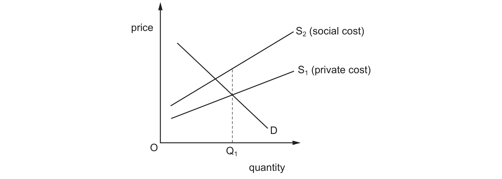
Answer: B.
The other options would each look different on the diagram. A subsidy (A) or a positive externality (C) would put the social curve BELOW the private one. A specific tax (D) shifts the private supply curve itself rather than opening a gap between two separate curves.
Question 2
The diagram shows the demand for and supply of a good and the marginal social costs (MSC) for that good. Assuming there are no external benefits, which area measures the net social benefit at output OQ?
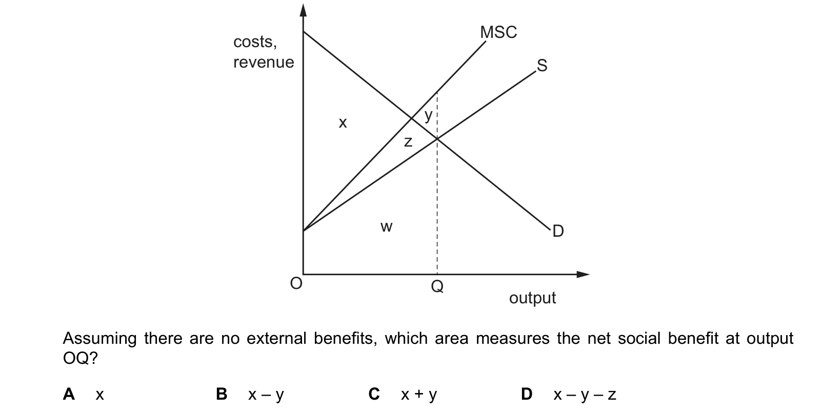
Answer: B.
Subtracting it once gives x minus y. A leaves the external cost out altogether, C adds it as though harm to third parties were a gain, and D takes off a further area on top, deducting more than the externality actually costs.
Question 3
The production of a firm which operates in an imperfectly competitive market gives rise to external production costs. Which statement about this firm must be correct?
Answer: C.
The other options all claim more than the question supports. Nothing has been said about external BENEFITS, so A cannot be judged either way. B reverses the relationship, which would need a negative external cost. D compares social cost with social benefit, which is a claim about whether output is too high, and that depends on the size of the externality rather than on its existence.
20. Final synthesis
The entire topic can be reduced to two marginal comparisons:
- private decisions generate market output where MPC = MPB;
- social efficiency requires output where MSC = MSB.
Externalities, information asymmetry and moral hazard explain why private incentives can diverge from social welfare. Cost–benefit analysis then provides a structured, but imperfect, method for comparing the full social consequences of decisions.
Related CIE 9708 topics
Not the topic you were looking for? Describe what you are stuck on in your own words and we will take you to the notes that answer it.